
Key points
- MAAT extends the 2022 Anomaly Transformer by swapping dense self attention for a windowed sparse attention mechanism and adding a Mamba state space branch inside the reconstruction stage.
- A learned gate decides, position by position, how much to trust the state space branch versus the original sparse attention output, rather than fusing them with a fixed rule.
- Across five widely used benchmarks, MSL, SMAP, SWaT, PSM, and SMD, MAAT posts the best F1 score on four of them and comes within half a point on the fifth.
- The efficiency story is the more interesting one. MAAT runs at 0.41 GFLOPs against DCdetector’s 3.58 GFLOPs on the same setup, roughly an order of magnitude difference.
- The ablation table tells a more complicated story than the headline numbers, and a couple of individual components actually make results worse before the gate learns to balance them.
Why finding the anomaly is harder than it sounds
Anomaly detection in a time series is a strange kind of problem because you almost never get to train on examples of the thing you are looking for. A factory does not hand you a labeled archive of every failure mode its machines might someday exhibit. So the whole field has leaned on unsupervised methods that learn what normal looks like and then treat anything that reconstructs poorly, or that behaves statistically differently from its neighbors, as suspicious.
The trouble is that normal itself is a moving target. A server cluster has daily load cycles. A Mars rover has mission phases. A water treatment plant has seasonal chemistry drift. Older tools such as ARIMA and Gaussian process models, built on the idea that deviations from a forecast are anomalies, tend to struggle once the underlying pattern gets nonlinear or high dimensional, which real industrial data almost always is. Reconstruction based deep models such as autoencoders improved on this but introduced a different failure mode, where anomalies that happen to resemble normal patterns slip through as false negatives, while noisy normal stretches get flagged as false positives.
From association discrepancy to a smarter kind of attention
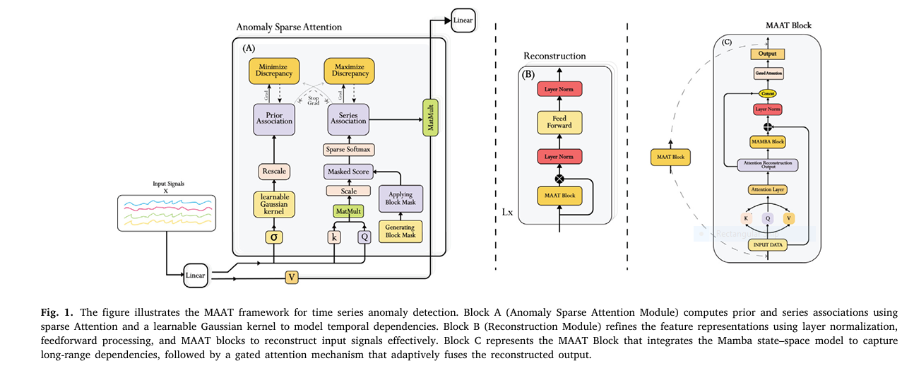
The 2022 Anomaly Transformer, proposed by Xu and colleagues, tried to sidestep the reconstruction only approach with an idea called association discrepancy. Instead of asking only how well a point reconstructs, the model compares two views of how each time step relates to its neighbors. One view, called the prior association, is modeled with a learnable Gaussian kernel that assumes nearby points matter more, the kind of assumption a human analyst would make instinctively. The other view, the series association, comes from ordinary self attention, learned directly from data. Anomalies, the reasoning goes, struggle to build a convincing series association because they lack the surrounding context that normal points have, so the gap between the two views becomes a detection signal.
That idea held up well, and it inspired DCdetector, from Yang and colleagues, which replaced the whole apparatus with a dual attention contrastive setup and dropped the Gaussian kernel entirely. DCdetector is elegant, but the MAAT authors point out a practical cost, its pairwise contrastive comparisons get expensive fast, which shows up later in the FLOPs comparison. Meanwhile the original Anomaly Transformer still leans on full self attention, which scales quadratically with sequence length and can lose track of long range structure inside a short context window. Separately, the Mamba line of work from Gu and Dao introduced selective state space models that scale linearly instead of quadratically, and had already shown strong results in language and audio tasks. MAAT is essentially the question of what happens if you let a linear time sequence model and a windowed attention mechanism share the reconstruction job, instead of asking one architecture to do everything.
How the architecture actually fits together
MAAT keeps the association discrepancy idea from the Anomaly Transformer but changes how the series association gets computed. Instead of full self attention over the whole window, each query position only attends to a local neighborhood defined by a block size parameter. Formally, for a query at position i, the model only normalizes attention scores over keys j where the distance between i and j is within half the block size. Everything outside that window gets a zero weight rather than a small nonzero one, which is the real source of the compute savings, since the softmax normalization itself only has to run over a fraction of the sequence.
That sparse series association still gets compared against the Gaussian kernel prior association through Kullback Leibler divergence in both directions, exactly as in the original formulation, which the paper writes as a sum over layers and time steps.
The second change happens deeper in the reconstruction stage. After sparse attention produces its output, that representation is fed through a Mamba block, which the authors describe as capturing longer range dependencies that a windowed attention mechanism, almost by definition, cannot see. Rather than simply replacing the attention output with the Mamba output, the architecture keeps both. The Mamba output is added back to the original pre attention representation through a residual connection and normalized, producing what the paper calls the skip path.
The interesting design decision is what happens next. Rather than averaging the skip path and the main path, or picking one architecturally, MAAT learns a gate from the concatenation of both, a small linear layer followed by a sigmoid, and uses that gate to blend the two element by element.
When the gate leans toward one, the model is effectively saying this segment needs the longer range context the Mamba branch provides. When it leans toward zero, the model trusts the locally focused sparse attention output more. The anomaly score itself then folds the association discrepancy together with the reconstruction error against this gated output, so a point only scores as suspicious if it both breaks the expected association pattern and reconstructs poorly under the model’s best combined effort.
Why the gate matters more than it looks
The paper’s own ablation shows that combining sparse attention and the Mamba branch without any gating mechanism actually performs worse than either component alone on some datasets. The gate is not decoration, it is what keeps two reasonable ideas from working against each other.
What the benchmarks actually show
The authors test MAAT against a long list of baselines, from classic methods such as isolation forest and one class support vector machines up through the modern transformer based approaches, across seven datasets that span aerospace telemetry, server infrastructure, industrial control systems, solar physics, and drinking water quality. The headline point based precision, recall, and F1 numbers on the five most common benchmarks are below, alongside the two strongest recent baselines.
| Dataset | Method | Precision | Recall | F1 |
|---|---|---|---|---|
| SMD | Anomaly Transformer | 88.47 | 92.28 | 90.33 |
| SMD | DCdetector | 85.82 | 84.10 | 84.95 |
| SMD | MAAT | 89.03 | 95.82 | 92.30 |
| MSL | Anomaly Transformer | 91.02 | 96.03 | 93.93 |
| MSL | DCdetector | 91.25 | 97.40 | 94.75 |
| MSL | MAAT | 92.06 | 98.33 | 95.05 |
| SMAP | Anomaly Transformer | 93.59 | 99.41 | 96.41 |
| SMAP | DCdetector | 94.29 | 97.97 | 96.10 |
| SMAP | MAAT | 94.75 | 99.33 | 96.99 |
| SWaT | Anomaly Transformer | 93.59 | 99.41 | 96.41 |
| SWaT | DCdetector | 93.12 | 99.96 | 96.42 |
| SWaT | MAAT | 93.33 | 100.00 | 96.50 |
| PSM | Anomaly Transformer | 97.14 | 97.81 | 97.47 |
| PSM | DCdetector | 97.22 | 98.45 | 97.83 |
| PSM | MAAT | 97.48 | 99.17 | 98.32 |
Notice the pattern across every dataset here, MAAT wins or ties on recall by a comfortable margin and only occasionally loses a fraction of a point on precision. That is a deliberate design outcome as much as a happy accident. In the aerospace and industrial control settings, a missed anomaly is far costlier than a false alarm an operator has to double check, so a model that trades a sliver of precision for meaningfully higher recall is doing the economically sensible thing, not just chasing a bigger number.
The efficiency comparison is where the sparse attention design pays off most clearly. On a matched setup, the original Anomaly Transformer uses 1.64 million parameters and 0.33 GFLOPs, replacing its attention with sparse attention alone drops that slightly to 1.59 million parameters and 0.31 GFLOPs, DCdetector needs only 0.91 million parameters but burns through 3.58 GFLOPs because of its pairwise contrastive comparisons, and full MAAT lands at 2.19 million parameters and 0.41 GFLOPs. In other words, MAAT is roughly nine times cheaper in compute than DCdetector while beating it on F1 across four of the five main benchmarks.
A separate stress test in the appendix isolates just the attention swap. On a synthetic spike anomaly, sparse attention needed 0.52 million floating point operations compared to full attention’s 5.12 million, a ninety percent reduction, and it produced a cleaner anomaly score that stayed under threshold during normal operation instead of drifting close to it. On a slower trend anomaly, the savings were similar, about eighty seven percent, and sparse attention also returned to baseline faster once the anomaly ended, while full attention lingered with an elevated score for several extra time steps.
What the ablation study quietly admits
This is the part of the paper worth reading closely, because it undercuts a simple story where every added component helps a little. On SMD, adding gating alone to the base Anomaly Transformer takes F1 from 90.33 to 91.05, a solid gain from a genuinely small change. Adding sparse attention alone, without gating or Mamba, actually drops F1 to 89.18, because the windowed formulation misses the multi machine correlations that matter in that dataset. Combining Mamba and sparse attention without any gate is worse still, an F1 of 87.02, the lowest score in the entire table for that dataset. Only once gating ties everything together does the full model reach 92.30.
That pattern, where the naive combination underperforms the individual pieces, repeats with variations across the other datasets. On PSM, sparse attention alone actually reaches 98.31 F1, nearly matching the full model’s 98.32, because PSM’s anomalies are short sharp spikes that a tightly local attention window is well suited to catch on its own. On NIPS TS GECCO, a sporadic anomaly water quality dataset, sparse attention alone hits an F1 of 58.82, actually higher than the full MAAT model’s 52.82, which the authors are upfront about, writing that the full architecture may be more model than this particular dataset needs. That kind of honesty in a results section is unusual and worth crediting, since it would have been easy to only report the datasets where every component helps.
The practical takeaway
If you are adapting this approach to your own sensor data, do not assume every module in the paper will help your specific case. The right combination looks like it depends heavily on whether your anomalies are short local spikes, in which case sparse attention alone may already be enough, or long slow drifts spread across correlated channels, where the Mamba branch earns its cost.
Where this fits in the broader shift toward linear time sequence models
MAAT is one instance of a pattern showing up across sequence modeling generally, hybridizing quadratic attention with linear time state space models rather than picking a side. The appeal is obvious on paper, Mamba’s selective scanning gives it linear scaling in sequence length and the paper cites throughput up to five times higher than a similarly sized transformer, while attention still offers the kind of fine grained, content addressable lookups that a purely recurrent state struggles to match. What MAAT adds to that general pattern is the specific claim that a learned gate, rather than a fixed architectural choice, should decide how much of each branch to trust at each position, and its ablation results are really an argument for why that gate is necessary rather than optional.
It is also a useful data point for anyone comparing time series work to the vision and language literature, where attention and selective state space hybrids have mostly been justified by throughput at very long context lengths. Here the context windows are only around one hundred time steps for most datasets in the paper, per the hyperparameter table, so the efficiency argument is less about handling millions of tokens and more about not paying full quadratic cost for local patterns the model does not need long range attention to see in the first place.
The clinical translation gap does not apply here
The paper’s introduction gestures at healthcare as one of several possible application areas for anomaly detection broadly, alongside finance and industrial monitoring, but none of the seven benchmark datasets involve patient data, diagnosis, or clinical outcomes. The datasets are NASA telemetry, a server infrastructure trace, a secure water treatment testbed, and two NIPS competition sets covering solar weather and drinking water quality. Readers coming from a medical AI background should treat this as a general purpose sequence modeling paper rather than a clinical one.
Honest limitations
The authors flag their own biggest caveat directly, the model is sensitive to how you balance the reconstruction module against the Mamba pathway, and tuning that balance is not automatic. The ablation results above make that concrete, since a poorly balanced combination of sparse attention and Mamba performs worse than either piece alone on more than one dataset.
On the SMAP dataset specifically, MAAT’s volume based ROC and precision recall metrics, 92.06 and 90.70, trail the plain Anomaly Transformer’s 95.52 and 93.77. The authors attribute this to SMAP’s long range, low noise telemetry pattern being a poor match for a block wise sparse attention mechanism that is tuned to suppress spurious correlations in noisier settings. That is a real tradeoff, not a minor rounding difference, and it means MAAT is not a universal upgrade over every prior method on every metric.
The paper also reports results on only seven datasets, all previously used in the Anomaly Transformer and DCdetector papers, which keeps the comparison fair but does not tell us how the model behaves on data with substantially different sampling rates, missing value patterns, or dimensionality than these seven benchmarks. And like most anomaly detection papers built around a fixed anomaly ratio threshold, the reported numbers assume you already know roughly what fraction of your data is anomalous, between 0.5 and 1 percent for most of these datasets according to the paper’s own hyperparameter table, which is a real world constraint worth sitting with before assuming the numbers transfer directly to a new deployment.
Conclusion
MAAT’s core achievement is showing that the association discrepancy idea behind the Anomaly Transformer does not require full quadratic self attention to work, and that a linear time state space branch can recover the long range context a windowed attention mechanism gives up, provided something is actually deciding how to weigh the two rather than assuming they always agree. The result is a model that matches or beats two strong prior architectures on four of five major benchmarks while running at a fraction of DCdetector’s compute cost, which matters enormously for anyone trying to deploy this kind of monitoring on infrastructure that already has enough sensors and enough data volume without adding a heavy inference bill on top.
The conceptual shift worth taking away is subtler than the leaderboard numbers suggest. Rather than treating attention and state space modeling as competing architectures where you pick a winner, MAAT treats them as specialists with different blind spots, sparse attention for sharp local events, Mamba for slow global drift, and lets a learned gate arbitrate between them per position. That framing generalizes well beyond anomaly detection, and it is easy to imagine the same skip and gate pattern showing up in forecasting, imputation, or classification architectures built on sequential data of any kind, not just the seven telemetry style datasets tested here.
The honest ablation results are, in a strange way, the most transferable part of the paper. They demonstrate that combining two reasonable architectural ideas without a mechanism to arbitrate between them can make results worse, not better, a lesson that applies well past this specific model and is easy to overlook when a paper only reports its best configuration.
The remaining limitations are real and worth restating plainly. Performance depends on getting the balance between the reconstruction branch and the Mamba pathway right for each dataset, the model underperforms the plain Anomaly Transformer on SMAP’s volume based metrics, and the evaluation, while broader than most papers in this space, still covers only seven datasets that were also used to benchmark the two closest prior methods.
Where this goes next probably depends on whether someone runs MAAT, or something like it, against sensor data with a genuinely different structure than these seven benchmarks, faster sampling rates, missing data, or many more channels than SWaT’s fifty one. Until then, the fair way to describe MAAT is as a well tested, computationally honest improvement on a specific architectural lineage, not a universal solution to anomaly detection, and that is a perfectly respectable place for a piece of research to land.
A working PyTorch implementation
The block below is a from scratch, runnable implementation of the architecture described above, built to match the equations in the paper rather than copied from any specific repository. It includes the sparse attention module, a simplified selective state space block standing in for the full Mamba library, the gated fusion layer, the association discrepancy loss with its minimax style alternation, an anomaly scoring function, and a smoke test on random data so you can confirm the shapes line up before pointing it at real sensor readings.
# maat_model.py
# A compact, runnable reimplementation of the MAAT architecture
# Sparse Attention + Mamba style state space block + Gated Attention fusion

import math
import torch
import torch.nn as nn
import torch.nn.functional as F


class SparseSeriesAttention(nn.Module):
    """Series association branch using block wise sparse attention."""

    def __init__(self, d_model, n_heads, block_size):
        super().__init__()
        self.d_model = d_model
        self.n_heads = n_heads
        self.block_size = block_size
        self.q_proj = nn.Linear(d_model, d_model)
        self.k_proj = nn.Linear(d_model, d_model)
        self.v_proj = nn.Linear(d_model, d_model)
        self.out_proj = nn.Linear(d_model, d_model)

    def _sparse_mask(self, seq_len, device):
        # mask[i, j] is True when j is inside i's local window
        idx = torch.arange(seq_len, device=device)
        dist = (idx.unsqueeze(0) - idx.unsqueeze(1)).abs()
        return dist <= (self.block_size // 2)

    def forward(self, x):
        B, N, D = x.shape
        Q = self.q_proj(x)
        K = self.k_proj(x)
        V = self.v_proj(x)

        scores = torch.matmul(Q, K.transpose(-2, -1)) / math.sqrt(D)
        mask = self._sparse_mask(N, x.device)
        scores = scores.masked_fill(~mask, float("-inf"))
        series = F.softmax(scores, dim=-1)
        out = torch.matmul(series, V)
        return self.out_proj(out), series


class GaussianPriorAssociation(nn.Module):
    """Prior association branch, a learnable Gaussian kernel over relative distance."""

    def __init__(self, d_model):
        super().__init__()
        self.sigma_proj = nn.Linear(d_model, 1)

    def forward(self, x):
        B, N, D = x.shape
        sigma = torch.sigmoid(self.sigma_proj(x)) * 5.0 + 1e-3
        idx = torch.arange(N, device=x.device).float()
        dist = (idx.unsqueeze(0) - idx.unsqueeze(1)).abs().unsqueeze(0)
        sigma_b = sigma.squeeze(-1).unsqueeze(1)
        prior = torch.exp(-(dist ** 2) / (2 * sigma_b ** 2))
        prior = prior / (prior.sum(dim=-1, keepdim=True) + 1e-8)
        return prior, sigma


class SelectiveStateSpaceBlock(nn.Module):
    """A simplified selective state space block in the spirit of Mamba.
    A full deployment should use the mamba_ssm package for the
    hardware aware parallel scan, this version uses a sequential
    scan so it stays dependency free and easy to read."""

    def __init__(self, d_model, d_state=16, d_conv=4):
        super().__init__()
        self.d_model = d_model
        self.d_state = d_state
        self.in_proj = nn.Linear(d_model, d_model * 2)
        self.conv = nn.Conv1d(d_model, d_model, kernel_size=d_conv,
                               padding=d_conv - 1, groups=d_model)
        self.x_proj = nn.Linear(d_model, d_state * 2 + d_model)
        self.a_log = nn.Parameter(torch.randn(d_model, d_state) * 0.1)
        self.out_proj = nn.Linear(d_model, d_model)

    def forward(self, x):
        B, N, D = x.shape
        x_res, gate = self.in_proj(x).chunk(2, dim=-1)
        x_conv = self.conv(x_res.transpose(1, 2))[:, :, :N].transpose(1, 2)
        x_conv = F.silu(x_conv)

        delta_b_c = self.x_proj(x_conv)
        delta, Bm, Cm = torch.split(
            delta_b_c, [D, self.d_state, self.d_state], dim=-1
        )
        delta = F.softplus(delta[..., :1]).expand(-1, -1, D)
        A = -torch.exp(self.a_log)

        state = torch.zeros(B, D, self.d_state, device=x.device)
        outputs = []
        for t in range(N):
            dA = torch.exp(delta[:, t].unsqueeze(-1) * A)
            dB = delta[:, t].unsqueeze(-1) * Bm[:, t].unsqueeze(1)
            state = state * dA + dB * x_conv[:, t].unsqueeze(-1)
            y_t = (state * Cm[:, t].unsqueeze(1)).sum(-1)
            outputs.append(y_t)
        y = torch.stack(outputs, dim=1)
        y = y * F.silu(gate)
        return self.out_proj(y)


class GatedFusion(nn.Module):
    """Adaptive gate that blends the skip path with the main path."""

    def __init__(self, d_model):
        super().__init__()
        self.gate_proj = nn.Linear(d_model * 2, d_model)

    def forward(self, x, x_skip):
        g = torch.sigmoid(self.gate_proj(torch.cat([x, x_skip], dim=-1)))
        return g * x_skip + (1 - g) * x, g


class MAATBlock(nn.Module):
    def __init__(self, d_model, n_heads, block_size, d_state=16, d_conv=4):
        super().__init__()
        self.sparse_attn = SparseSeriesAttention(d_model, n_heads, block_size)
        self.prior_assoc = GaussianPriorAssociation(d_model)
        self.mamba = SelectiveStateSpaceBlock(d_model, d_state, d_conv)
        self.gate = GatedFusion(d_model)
        self.norm_skip = nn.LayerNorm(d_model)
        self.norm_out = nn.LayerNorm(d_model)
        self.ffn = nn.Sequential(
            nn.Linear(d_model, d_model * 4),
            nn.GELU(),
            nn.Linear(d_model * 4, d_model),
        )

    def forward(self, x):
        x_orig = x
        attn_out, series = self.sparse_attn(x)
        prior, sigma = self.prior_assoc(x)

        x_mamba = self.mamba(attn_out)
        x_skip = self.norm_skip(x_mamba + x_orig)

        fused, g = self.gate(attn_out, x_skip)
        fused = fused + self.ffn(fused)
        out = self.norm_out(fused)
        return out, series, prior, sigma


class MAAT(nn.Module):
    def __init__(self, n_features, d_model=512, n_heads=8,
                 n_layers=3, block_size=16, d_state=16, d_conv=4):
        super().__init__()
        self.embed = nn.Linear(n_features, d_model)
        self.layers = nn.ModuleList([
            MAATBlock(d_model, n_heads, block_size, d_state, d_conv)
            for _ in range(n_layers)
        ])
        self.reconstruct = nn.Linear(d_model, n_features)

    def forward(self, x):
        h = self.embed(x)
        series_list, prior_list, sigma_list = [], [], []
        for layer in self.layers:
            h, series, prior, sigma = layer(h)
            series_list.append(series)
            prior_list.append(prior)
            sigma_list.append(sigma)
        recon = self.reconstruct(h)
        return recon, series_list, prior_list, sigma_list


def association_discrepancy(series_list, prior_list, eps=1e-8):
    """Equation 2, symmetric KL divergence averaged over layers."""
    total = 0.0
    L = len(series_list)
    for series, prior in zip(series_list, prior_list):
        p = prior.clamp_min(eps)
        s = series.clamp_min(eps)
        kl_ps = (p * (p / s).log()).sum(-1)
        kl_sp = (s * (s / p).log()).sum(-1)
        total = total + (kl_ps + kl_sp).sum(-1)
    return total / L


def maat_loss(x, recon, series_list, prior_list, lam=3.0, phase="minimize"):
    """Minimax style loss following the Anomaly Transformer strategy.
    In the minimize phase the prior is trained to match a detached
    series association. In the maximize phase the series is trained
    to move away from a detached prior."""
    recon_loss = F.mse_loss(recon, x)

    detached_series = [s.detach() for s in series_list]
    detached_prior = [p.detach() for p in prior_list]

    if phase == "minimize":
        assdis = association_discrepancy(detached_series, prior_list).mean()
        return recon_loss - lam * assdis
    else:
        assdis = association_discrepancy(series_list, detached_prior).mean()
        return recon_loss + lam * assdis


def anomaly_score(x, recon, series_list, prior_list):
    """Equation 10, association discrepancy combined with reconstruction error."""
    assdis = association_discrepancy(series_list, prior_list)
    weight = F.softmax(-assdis, dim=-1)
    point_error = ((x - recon) ** 2).sum(-1)
    return weight * point_error


def train_step(model, optimizer, x):
    optimizer.zero_grad()
    recon, series_list, prior_list, _ = model(x)

    loss_min = maat_loss(x, recon, series_list, prior_list, phase="minimize")
    loss_min.mean().backward(retain_graph=True)

    recon2, series_list2, prior_list2, _ = model(x)
    loss_max = maat_loss(x, recon2, series_list2, prior_list2, phase="maximize")
    loss_max.mean().backward()

    optimizer.step()
    return loss_min.mean().item(), loss_max.mean().item()


def evaluate(model, x, anomaly_ratio=0.01):
    model.eval()
    with torch.no_grad():
        recon, series_list, prior_list, _ = model(x)
        scores = anomaly_score(x, recon, series_list, prior_list)
    flat = scores.flatten()
    k = max(1, int(len(flat) * anomaly_ratio))
    threshold = torch.topk(flat, k).values.min()
    predictions = (scores >= threshold).long()
    return scores, predictions, threshold.item()


if __name__ == "__main__":
    # smoke test on random dummy data, confirms shapes and a working forward and backward pass
    torch.manual_seed(0)
    batch_size, seq_len, n_features = 4, 100, 25

    model = MAAT(n_features=n_features, d_model=128, n_heads=4,
                 n_layers=2, block_size=16, d_state=8, d_conv=4)
    optimizer = torch.optim.Adam(model.parameters(), lr=1e-4)

    dummy_x = torch.randn(batch_size, seq_len, n_features)

    loss_min, loss_max = train_step(model, optimizer, dummy_x)
    print(f"minimize phase loss {loss_min:.4f}")
    print(f"maximize phase loss {loss_max:.4f}")

    scores, predictions, threshold = evaluate(model, dummy_x, anomaly_ratio=0.05)
    print(f"anomaly score shape {tuple(scores.shape)}")
    print(f"flagged points {int(predictions.sum().item())} out of {predictions.numel()}")
    print(f"threshold {threshold:.6f}")
Frequently asked questions
What does MAAT actually stand for and what problem is it solving
MAAT stands for Mamba Adaptive Anomaly Transformer. It is built to find unusual points in a time series, such as a sensor spike or a slow drift toward an abnormal state, without needing labeled examples of failures during training.
How is MAAT different from the original Anomaly Transformer
It replaces the original’s dense self attention with a windowed sparse attention mechanism and adds a Mamba style state space branch inside the reconstruction stage, with a learned gate deciding how much to rely on each branch at every position.
Does MAAT beat DCdetector on every dataset
Not on every metric. It wins or ties on F1 across most of the five main benchmarks and uses far less compute, but DCdetector edges it out on a couple of precision related metrics on MSL and SMAP.
Is MAAT faster than DCdetector
Yes by a wide margin. The paper reports 0.41 GFLOPs for MAAT against 3.58 GFLOPs for DCdetector on a matched setup, close to a ninefold difference, largely because DCdetector relies on expensive pairwise contrastive comparisons.
What datasets was MAAT tested on
Seven benchmarks covering NASA Mars rover telemetry, soil moisture satellite data, a server infrastructure trace, a secure water treatment testbed, an eBay server metrics set, solar weather magnetograms, and a drinking water quality dataset.
Can I use this on my own sensor data
The architecture is domain agnostic and the paper’s own code repository plus the implementation above give a starting point, but the ablation results show performance depends heavily on tuning the balance between the sparse attention and Mamba branches for your specific data pattern.
Sellam, A. Z., Benaissa, I., Taleb Ahmed, A., Patrono, L., and Distante, C. Mamba Adaptive Anomaly Transformer with association discrepancy for time series. Engineering Applications of Artificial Intelligence, 160, 111685, 2025. https://doi.org/10.1016/j.engappai.2025.111685
This analysis is based on the published paper and an independent evaluation of its claims.