
Key points
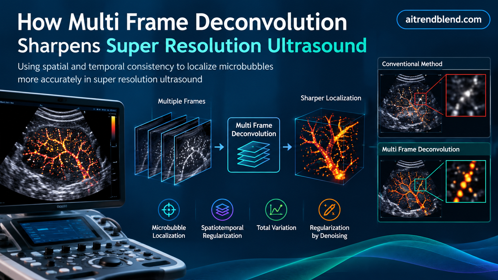
- The paper introduces a framework called Multi Frame Deconvolution, or MF Decon, that processes a whole stack of ultrasound frames together instead of one frame at a time.
- Two new methods come out of that framework, MF Decon plus 3DTV and MF Decon plus RED plus TV, each combining a spatial noise filter with a temporal one built for how microbubbles actually move.
- On simulated data with known ground truth, the new methods raised precision by as much as 39 percent over normalized cross correlation and recall by up to 12 percent.
- On real rat brain scans, the resulting vessel maps showed a contrast to noise ratio of 25.65 decibels for MF Decon plus 3DTV against 16.53 decibels for the older cross correlation approach.
- The trade off is time. The new methods take roughly four times as long to run as ordinary deconvolution on the same GPU hardware.
Why finding a microbubble in a noisy image is harder than it sounds
Super resolution ultrasound, also called ultrasound localization microscopy, works by injecting a patient or an animal with microbubble contrast agents and then watching where those bubbles go as blood carries them through the smallest vessels in an organ. Each bubble shows up as a bright blob in the ultrasound image, and if you can pin down its exact position across hundreds or thousands of frames, you can trace out vessels far smaller than a conventional ultrasound scan could ever resolve. The technique has already been used to image the microvasculature of the rat brain, the rabbit kidney, the human breast, the human liver, and even a beating human heart, among the many applications the paper cites.
The catch is that localizing a bubble accurately depends on being able to tell a real microbubble apart from noise, and contrast enhanced ultrasound images are noisy by nature. The authors point out that the noise in beamformed ultrasound data follows a Rician distribution, which in practice behaves a lot like Gaussian noise once the signal to noise ratio gets low. Standard approaches such as peak detection or centroid finding after background removal are prone to mistaking a bright noise spike for a bubble. Normalized cross correlation against an estimated point spread function helps, but it struggles when two bubbles sit close together, because correlating with a blurry point spread function produces an even blurrier correlation map. Deconvolution methods do better at separating overlapping bubbles because they try to reverse the blur mathematically rather than just matching a template, but on their own they are still vulnerable to noise corrupting the result frame by frame.
The idea that a stack of frames carries more information than any single frame
Here is the observation that drives the whole paper. A single acquisition in super resolution ultrasound is not one image, it is hundreds of images captured in quick succession, and those images are not independent of each other. A microbubble that shows up at one pixel does not vanish and reappear randomly, it rises from baseline, peaks, and fades as it passes through the field of view, and the shape of that rise and fall depends on how fast the bubble is moving. A fast bubble produces a sharp brief spike at a given pixel. A slow one produces a wider, gentler bump. Noise, by contrast, tends to flicker erratically from frame to frame with no such pattern.
Most existing localization pipelines throw that temporal structure away. They deconvolve or correlate each frame on its own and only start thinking about time once they move to the tracking stage, where bubbles get linked into trajectories after localization is already finished. The Imperial College team built a framework that instead treats the whole three dimensional block of data, two spatial dimensions plus time, as a single object to be deconvolved together, so that the noise removal step itself can use the temporal consistency of real bubble signals as a clue about what is signal and what is noise.
Takeaway
The central design choice in this paper is not a new denoising filter or a smarter detector. It is a decision to stop treating each ultrasound frame as its own isolated problem and instead solve one larger optimization across an entire stack of frames at once, adding a penalty term that rewards temporal smoothness the same way classic total variation rewards spatial smoothness.
How the deconvolution problem is actually set up
The starting point is the standard image formation model used across the field. A measured contrast enhanced ultrasound image Y is treated as the true, high resolution bubble distribution X convolved with the system point spread function A, plus additive noise E. The point spread function itself is estimated in a fairly hands on way, by manually picking around ten well separated bubbles from the data and fitting a two dimensional Gaussian to their average shape.
Recovering X from Y is an inverse problem, and because microbubble concentrations are typically sparse, meaning most pixels contain no bubble at all, the authors add an L1 norm penalty that encourages sparsity in the recovered image, along with a positivity constraint since intensity values cannot be negative. That gives the classic deconvolution objective used by earlier methods such as SUSHI and the fast iterative shrinkage thresholding algorithm approaches cited throughout the introduction.
The multi frame version simply extends every one of those variables from a two dimensional image to a three dimensional tensor stacking width, height, and time, with the same point spread function convolved slice by slice across every frame. On its own that already lets all frames be optimized jointly and lets the paper introduce a clever multi frame thresholding step, where the adaptive threshold used to pick out bubbles after deconvolution is averaged across all frames rather than recomputed separately for each one. The real contribution, though, is what gets added on top of that joint formulation.
Two flavors of regularization, one spatial and one temporal
The full objective adds two extra penalty terms, a spatial regularizer applied within each frame and a temporal regularizer applied across frames.
For the spatial term, the paper offers two choices. The first method, called MF Decon plus 3DTV, uses classic two dimensional total variation, the same idea Rudin, Osher, and Fatemi introduced back in 1992 for removing noise while keeping real edges intact. The second method, MF Decon plus RED plus TV, swaps that out for a technique called regularization by denoising, a framework from Romano, Elad, and Milanfar that lets you plug in essentially any off the shelf image denoiser and use it as a mathematically grounded regularizer inside an inverse problem. The authors chose a simple five by five median filter as their denoiser, reasoning that median filtering is cheap, has already proven useful in the post processing stage of other ultrasound localization pipelines, and preserves edges while smoothing noise, which is exactly what a regularizer needs to do here.
For the temporal term, both methods use one dimensional total variation applied along the time axis at each pixel. The intuition is the same one described earlier. A genuine bubble signal changes smoothly over a handful of frames as the bubble enters, peaks, and exits a given location, while noise jitters unpredictably, so penalizing rapid temporal change should suppress the noise while leaving real bubble trajectories mostly untouched.
Solving it without getting stuck in slow inner loops
Optimization problems with several regularizers like this are usually solved with the alternating direction method of multipliers, but standard ADMM often needs an inner gradient descent loop to update the main variable at each outer iteration, which is slow. The authors instead use a variant called inner loop free ADMM, first proposed by Donati, Soubies, and Unser for cryo electron microscopy reconstruction, which lets the main update be solved in one shot using the fast Fourier transform because convolution turns into simple multiplication in the frequency domain. That single design choice is a large part of why the method is fast enough to be practical on real GPU hardware, even though it is still solving a much bigger optimization problem than ordinary single frame deconvolution.
Practically, each iteration cycles through updating a set of auxiliary variables with proximal operators, soft thresholding for the sparsity term, a positivity clamp for the non negativity constraint, and either a total variation shrinkage step or an iterative median filtering step depending on which spatial regularizer is in play, then solves for the main deconvolved tensor in the frequency domain, then updates the dual variables that keep everything consistent. The whole loop runs for 500 iterations with a learning rate of 20 in the reported experiments.
What happened when they tested it on simulated data with known answers
Because you cannot verify localization accuracy against physical ground truth in a living animal, the authors first tested everything on a simulated dataset called BUFF, short for Bubble Flow Field, which was also used in the ULTRA SR localization and tracking challenge held at the 2022 IEEE International Ultrasonics Symposium. The simulation used parameters matching a high frequency L11-4 linear array transducer at 7.24 megahertz with three angle plane wave compounding and a 50 hertz post compounding frame rate, with realistic bandwidth filtered noise added to the raw channel data before beamforming.
They compared four methods head to head, normalized cross correlation, traditional single frame deconvolution, and their two new multi frame methods, at three noise levels corresponding to signal to noise ratios of 15, 10, and 5 decibels. A localized bubble counted as a true positive if it landed within half a wavelength of a ground truth position.
| SNR | Method | Precision | Recall | Mean error, micrometers | F1 score |
|---|---|---|---|---|---|
| 15 dB | NCC | 0.661 | 0.412 | 45.28 | 0.508 |
| 15 dB | Decon | 0.859 | 0.557 | 37.47 | 0.676 |
| 15 dB | MF Decon plus 3DTV | 0.890 | 0.566 | 37.27 | 0.692 |
| 15 dB | MF Decon plus RED plus TV | 0.869 | 0.566 | 36.69 | 0.686 |
| 5 dB | NCC | 0.379 | 0.219 | 54.24 | 0.278 |
| 5 dB | Decon | 0.451 | 0.282 | 49.67 | 0.347 |
| 5 dB | MF Decon plus 3DTV | 0.551 | 0.285 | 48.18 | 0.375 |
| 5 dB | MF Decon plus RED plus TV | 0.495 | 0.287 | 48.47 | 0.363 |
A few patterns jump out. Both new methods beat cross correlation and traditional deconvolution at every noise level on precision, recall, F1 score, and localization error. The gap actually widens as the data gets noisier, which is a genuinely useful property since noise is the whole reason this kind of method matters in the first place. Given the same number of localized bubbles, MF Decon plus 3DTV localized up to 12 percent more real bubbles than cross correlation and 5 percent more than ordinary deconvolution, and at matched recall it placed bubbles up to 39 percent closer to their true positions than cross correlation and 15 percent closer than deconvolution. The RED based variant landed a little behind 3DTV on these simulated numbers but still comfortably ahead of both older methods.
Moving from simulation to a real rat brain
Simulated bubbles behave exactly the way your model expects them to, which is precisely why the second half of the evaluation matters more. The authors turned to a publicly available in vivo rat brain dataset originally collected for a different paper by Shin and colleagues, built around a high frequency L22-14vX transducer running at 15.625 megahertz with five angle plane wave compounding and a punishing 1000 hertz post compounding frame rate, totaling 20000 frames across 80 separate ten second acquisitions. Tissue background was removed with singular value decomposition based clutter filtering, and because the rat was fixed in a stereotaxic frame, motion correction was not needed.
Since there is no ground truth for a living brain, the comparison strategy shifts. The team made sure every method localized the same total number of bubbles, then fed those localizations into an identical tracking algorithm, on the reasoning that if two methods detect the same number of bubbles, the one producing cleaner, more consistent localizations should generate better connected vessel trajectories and a visually sharper vessel map.
That is exactly what happened. The contrast to noise ratio measured in a fixed region of the resulting vessel density maps came out at 16.53 decibels for cross correlation, 21.26 for ordinary deconvolution, 25.65 for MF Decon plus 3DTV, and 21.64 for MF Decon plus RED plus TV. Image resolution, measured with Fourier ring correlation at the standard half bit threshold, improved from 31.65 micrometers for cross correlation down to 24.21 micrometers for MF Decon plus 3DTV, both comfortably below the 49.28 micrometer half wavelength limit that defines conventional resolution for this transducer.
Longer vessel trajectories, which is where the tracking algorithm actually benefits
Perhaps the most concrete downstream number in the paper concerns trajectory length. Once localizations from each method were passed through the same bubble tracking algorithm, the average tracked trajectory length came out at 3.91 frames for cross correlation, 4.40 frames for ordinary deconvolution, 6.98 frames for MF Decon plus 3DTV, and 8.90 frames for MF Decon plus RED plus TV. That last number represents more than double the trajectory length achieved by cross correlation. A one way ANOVA across the four groups produced a p value of 4.87 times ten to the negative 149, and a Tukey honestly significant difference post hoc test confirmed every pairwise difference was significant at p less than 0.001. Longer trajectories matter because the tracking step is what turns individual bubble positions into continuous vessel segments, so cleaner, longer tracks translate directly into more complete and more legible microvasculature maps, which is visible in the paper’s side by side comparisons where vessels that are barely discernible under cross correlation or ordinary deconvolution appear as clear, continuous structures under the new methods.
Takeaway
The improvement is not just a cosmetic denoising effect. It changes what the downstream tracking algorithm is able to do, because localization quality feeds directly into how confidently bubbles can be linked across frames into coherent vessel paths, and a noisier localization stage tends to break tracks apart rather than just adding a little jitter to them.
What it costs, and where it might struggle
None of this comes for free. On an AMD Ryzen 9 5950X paired with an NVIDIA RTX 4090 GPU, deconvolving a 450 by 650 pixel volume across 250 frames took 9.35 minutes for MF Decon plus 3DTV and 8.24 minutes for MF Decon plus RED plus TV, compared with 2.29 minutes for ordinary deconvolution and 4.82 minutes for cross correlation running on CPU. That is a real cost for anyone processing large datasets, though the authors note their tensor based formulation is well suited to GPU acceleration, which is part of why the runtime stays in the single digit minutes rather than ballooning further.
There are also more hyperparameters to manage than with the simpler baseline methods, weights controlling the sparsity term, the spatial regularizer, and the temporal regularizer, plus ADMM penalty coefficients for each constraint. The paper offers practical guidance rather than a fixed recipe. A stronger spatial constraint helps when noise is heavy but risks smoothing away fine detail if pushed too far. A stronger temporal constraint helps when bubbles move slowly and frame rates are high, since consecutive frames then carry a lot of shared information, while a weaker temporal constraint suits fast moving bubbles captured at low frame rates, since in that regime a bubble signal barely overlaps between consecutive frames and there is little temporal correlation left to exploit. In the most extreme case, where the frame rate is too low relative to bubble speed, the authors acknowledge the temporal regularizer may not help localization at all, though they note this scenario is uncommon in practice because the microvascular structures typically targeted by this kind of imaging tend to carry slow flow.
Two further limitations are worth flagging plainly. The method assumes the point spread function stays constant across the whole field of view, which is rarely exactly true, and the authors suggest dividing large images into smaller sub blocks with their own locally estimated point spread function as a workaround, an approach described in their earlier 2024 work. The deconvolution also introduces artifacts near the edges of the imaged region, because a bubble shape gets cropped when it sits at the boundary, which the authors say is usually manageable simply by cropping the region of interest away from the image edges.
The clinical translation gap
It is worth being direct about the distance between this result and anything resembling routine clinical use. Both evaluations here used a fixed, sedated, or stereotaxically immobilized animal or a controlled simulation, not a moving human patient in a clinical ultrasound suite. The rat brain dataset involved negligible tissue motion by design, and none of the reported experiments grapple with the added complexity of cardiac or respiratory motion that a human abdominal or cardiac scan would introduce. The point spread function estimation step is also manual, requiring an operator to pick out roughly ten well separated bubbles per acquisition, which is a workable step in a research pipeline but is not yet the kind of fully automated process a clinical workflow would need. None of this diminishes the algorithmic contribution, but it does mean the appropriate reading of this paper is as a meaningful advance in the imaging processing toolkit used by ultrasound researchers, not as a clinically validated diagnostic method ready for hospital deployment.
Where this fits in the broader super resolution ultrasound picture
The paper situates itself carefully against prior attempts to use temporal information in bubble localization, noting that only a handful of earlier papers explored this direction. Solomon and colleagues used the flow kinematics of individual bubbles as extra sparsity weights inside a deconvolution problem. A 2023 track and localize workflow from Leconte and colleagues flipped the usual order of operations, tracking probable bubble trajectories first and then refining localization based on those tracks. The LOCA-ULM network from Shin and colleagues, whose rat brain dataset gets reused here, took a deep learning route, localizing bubbles from three adjacent frames at once with a trained network. What sets this paper apart is that it builds temporal consistency directly into the mathematical regularization of a classical optimization based deconvolution problem, rather than relying on a separate tracking heuristic or a trained neural network whose behavior can be harder to characterize and whose performance depends heavily on how representative its training data was, an issue the introduction calls out as a real barrier to using learned models in clinical settings where ground truth is scarce.
The authors are also candid that the regularization by denoising framework opens a door they have only partly walked through. They chose a simple median filter as their denoiser mainly for speed and because it is already established in ultrasound post processing, but RED is explicitly built to accept any denoiser, and the paper name checks several deep learning based alternatives, including TNRD, DnCNN, and DRUNet, as plausible upgrades for a future version of the spatial regularizer. They also point out that nothing in the mathematics restricts this to two dimensional imaging, and that the same framework should extend to three dimensional ultrasound localization microscopy performed with matrix array or row column array probes, just with an extra spatial dimension threaded through the same convolutions.
Limitations, reported plainly
Summarizing the constraints the authors themselves acknowledge helps set realistic expectations for anyone considering the method for their own pipeline.
- Processing time runs roughly four times longer than standard deconvolution on the same GPU, and far longer than cross correlation running on CPU, which matters for datasets spanning tens of thousands of frames.
- The method carries more hyperparameters than the baselines it is compared against, and while the paper gives sensible tuning heuristics, getting the balance right for a new imaging setup will likely require some experimentation.
- The point spread function is assumed constant across the field of view, an assumption that can break down over a large imaging depth and that the authors address only by suggesting sub block processing rather than solving directly within this framework.
- Temporal regularization loses its benefit when frame rate is low relative to bubble speed, since consecutive frames then share little useful overlap.
- Both evaluations relied on simulation and animal data, with sample sizes of one simulated dataset across three noise levels and one 80 acquisition rat brain dataset, and the authors themselves note their cross correlation reimplementation produced different results from the original Shin and colleagues paper, a reminder that implementation details matter and that independent replication would strengthen confidence in the reported margins.
Complete PyTorch implementation of MF Decon plus 3DTV
The code below reimplements the inner loop free ADMM solver described in the paper for the MF Decon plus 3DTV method, built around equations 9 through 16 and Algorithm 1. It runs the full multi frame deconvolution on a synthetic stack of frames so you can see the mechanics end to end, including the sparsity thresholding, the positivity clamp, the spatial and temporal total variation proximal steps, and the frequency domain update for the main variable.
Two things are worth being upfront about if you plan to adapt this. First, the code above collapses the spatial derivative kernel handling into a single reusable helper for clarity, while the paper’s Algorithm 1 keeps three separate proximal updates, so treat this as a readable reference implementation rather than a byte for byte port. Second, the RED based variant, MF Decon plus RED plus TV, swaps the second spatial proximal step for the iterative median filter update in equation 18, which is straightforward to add with a few lines calling a median filter function inside the same loop, but is left out here to keep the smoke test simple.
The bigger picture
What makes this paper worth reading beyond its immediate numbers is the argument it makes about where the next real gains in super resolution ultrasound are likely to come from. A lot of recent work in the field has chased better neural network architectures for bubble detection, and those networks can handle high bubble concentrations well, but the authors are candid that their performance depends heavily on training data that matches the deployment setting, which is a genuine obstacle for clinical use where labeled ground truth barely exists. This paper takes a different route, staying inside a classical, mathematically interpretable optimization framework and finding real performance gains simply by being more honest about the structure already present in the data, namely that consecutive frames are not independent observations.
That framing has a kind of quiet ambition to it. The conceptual shift is not really about ultrasound at all, it is about recognizing that many imaging problems treated as a sequence of independent two dimensional reconstructions are secretly three or four dimensional problems in disguise, and that solving them jointly can recover information that gets lost when each frame is processed alone. The same logic shows up in cryo electron microscopy, in video super resolution, and in dynamic MRI reconstruction, and the inner loop free ADMM solver borrowed here for speed originally came from the cryo EM literature, which is itself a small piece of evidence for how portable this kind of thinking is across imaging fields.
The honest remaining limitations are the ones already discussed, the added compute cost, the manual point spread function estimation, the assumption of a spatially constant point spread function, and the gap between a fixed rat brain and a moving human patient. None of those are small, and closing them will take real engineering work rather than a single follow up experiment. The paper’s own suggestions for what comes next, extending the framework to three dimensional probes, trying higher order total variation, and swapping the simple median filter denoiser for a learned one such as DnCNN or DRUNet, all point toward a method that is still early in its development rather than a finished product.
Whether this specific combination of spatial and temporal regularizers becomes the standard approach or gets superseded by a learned equivalent within a couple of years is genuinely an open question. What seems more durable is the underlying insight, that the temporal dimension of contrast enhanced ultrasound data is not just something to exploit after localization during tracking, but something worth building into the localization step itself. If that idea holds up across more datasets and more imaging setups, it is likely to show up again in future ultrasound localization microscopy papers regardless of whether they keep the exact optimization machinery used here.
For a lab already running a deconvolution based ULM pipeline, the practical takeaway is straightforward even if the implementation is not trivial. Stacking frames and adding a temporal total variation term is a comparatively contained modification to an existing deconvolution codebase, and the reported gains, particularly the more than doubled average trajectory length on real brain data, are large enough to justify the extra GPU time for applications where imaging quality matters more than turnaround speed, such as detailed preclinical microvasculature studies rather than rapid bedside screening.
Frequently asked questions
What is Multi Frame Deconvolution or MF Decon in this paper
MF Decon is a framework that deconvolves a whole stack of contrast enhanced ultrasound frames together instead of processing each frame on its own, so that noise removal can take advantage of how a real microbubble signal changes smoothly over time while noise does not.
How is MF Decon plus 3DTV different from MF Decon plus RED plus TV
Both methods share the same multi frame deconvolution structure and the same one dimensional temporal total variation term. They differ only in how they clean up noise within each individual frame, with 3DTV using classic two dimensional total variation and RED plus TV using a regularization by denoising approach built around a five by five median filter.
How much better is this than normalized cross correlation
On simulated data with known ground truth, MF Decon plus 3DTV localized up to 12 percent more real microbubbles than normalized cross correlation at the same total number of detections, and placed bubbles up to 39 percent closer to their true positions at matched recall. On real rat brain data, the contrast to noise ratio of the resulting vessel maps improved from 16.53 decibels with cross correlation to 25.65 decibels with MF Decon plus 3DTV.
Does this method work on human data or only on animals
The paper evaluates the method on a simulated dataset and on a publicly available in vivo rat brain dataset. It has not been tested on human patients in this paper, and the authors themselves discuss remaining gaps, such as the manual point spread function estimation step and the assumption of little to no tissue motion, that would need addressing before clinical use.
What does the extra accuracy cost in processing time
On an RTX 4090 GPU, deconvolving a 450 by 650 pixel volume across 250 frames took 9.35 minutes for MF Decon plus 3DTV and 8.24 minutes for MF Decon plus RED plus TV, compared with 2.29 minutes for ordinary single frame deconvolution and 4.82 minutes for cross correlation on CPU.
Can this framework be extended to three dimensional ultrasound imaging
The authors state the underlying mathematics does not depend on staying in two dimensions and that the framework should extend to three dimensional ultrasound localization microscopy performed with matrix array or row column array probes, though that extension is proposed as future work rather than something tested in this paper.
Read the full peer reviewed paper for the complete mathematical derivation, the ADMM algorithm listings, and the supplementary figures referenced throughout this article.
Read the paperThis analysis is based on the published paper and an independent evaluation of its claims.
Pingback: 7 Shocking Wins and Pitfalls of Self-Distillation Without Teachers (And How to Master It!) - aitrendblend.com