Sticky Brownian Motion — The Complete Trivariate Distribution, Finally Written Down Correctly | AI Trend Blend

Probability Theory · Journal of Mathematical Analysis and Applications 560 (2026) · Universidade Nova de Lisboa & Université de Lorraine · 12 min read

A Particle That Gets Stuck — The Complete Mathematical Story of Sticky Brownian Motion, Finally Told Correctly

Two mathematicians from Portugal and France have derived a precise, closed-form formula that fully describes where sticky Brownian motion is, how long it has spent glued to the origin, and how much of its time it has passed on the positive side — simultaneously, in one elegant expression that corrects errors made in earlier work.

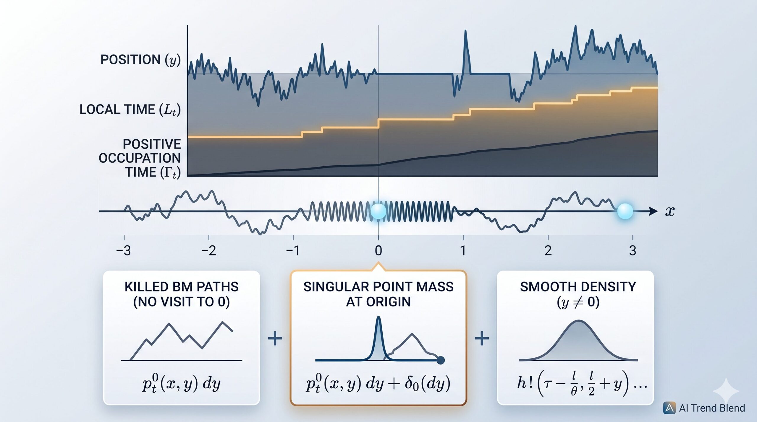
Sticky Brownian Motion Trivariate Distribution Local Time Occupation Time Laplace Transform Feller Diffusion Large Deviations Wasserstein Gradient Flow

Imagine a particle wandering randomly along a number line — diffusing left and right like smoke in still air, perfectly Brownian in character. Now give that particle one peculiar habit: whenever it reaches the point zero, instead of bouncing through immediately, it lingers. It gets sticky. It spends a measurable, positive amount of time parked at the origin before drifting away again. This is sticky Brownian motion, first described by William Feller in the 1950s and quietly influential ever since. A new paper by Jean-Baptiste Casteras and Léonard Monsaingeon now writes down, with complete precision, the full joint probability distribution of three quantities associated with this process — and in doing so, fixes genuine mistakes that had been sitting in the published literature for years.

What Is Sticky Brownian Motion, and Why Does It Matter?

Standard Brownian motion is the mathematician’s idealized random walk — continuous paths, Gaussian increments, no preferred direction. It is a foundational object in probability theory, appearing in financial models, physics, biology, and the study of partial differential equations. But standard Brownian motion passes through any single point instantaneously; it has zero probability of spending a positive amount of time at any fixed location. Its behavior at a boundary or special point is, in a precise sense, fleeting.

Sticky Brownian motion breaks this rule in the mildest possible way. Outside the origin, it behaves exactly like standard Brownian motion — same increments, same diffusion coefficient, same law. But at the origin, something different happens. The process can spend positive time there, proportional to how long it “wants” to stay based on a parameter $\theta > 0$ called the stickiness coefficient. The larger $\theta$, the more time the particle spends stuck at zero relative to its local time there.

Feller introduced this object in the 1950s as part of a systematic classification of all possible boundary behaviors for one-dimensional diffusions. His framework, developed through a series of papers on semi-groups and generators, identified sticky behavior as one of the canonical possibilities — alongside reflection, absorption, and periodic boundary conditions. For decades, sticky diffusions were something of a mathematical curiosity, studied primarily for their theoretical interest. That changed in recent years, as researchers found sticky processes appearing naturally in models of particle aggregation, interface dynamics, filtering theory, and numerical methods for constrained stochastic systems.

The Stickiness Coefficient in Plain Language

The parameter $\theta > 0$ controls exactly how “sticky” the origin is. When $\theta$ is very large, the particle barely pauses at zero — it is almost standard Brownian motion. When $\theta$ is very small, the particle spends a disproportionately long time at the origin, effectively getting trapped there for stretches of time. The ratio of time at zero to local time accumulated there is always exactly $1/\theta$.

Three Numbers That Describe Where the Particle Has Been

To fully understand where a sticky Brownian motion $S_t$ is and what it has experienced up to time $t$, you need more than just its current position. You need a complete accounting of its history with the special point at the origin. The paper tracks three quantities simultaneously:

The first is simply the position $y \in \mathbb{R}$ — where is the particle right now? For standard Brownian motion, this alone tells you everything. For sticky Brownian motion, position alone is not enough.

The second is the local time $L_t$ at the origin. Local time is one of the subtler objects in probability theory. Formally, it measures how much time the process has spent in an infinitesimally thin neighborhood of zero, normalized appropriately:

Local Time at the Origin $$L_t(S) := \lim_{\varepsilon \to 0} \frac{1}{2\varepsilon}\int_0^t \mathbf{1}_{[-\varepsilon,+\varepsilon]}(S_u)\,du = \theta \int_0^t \mathbf{1}_{\{S_u = 0\}}\,du.$$

The second equality — that this limit equals $\theta$ times the actual time spent at zero — is a deep and non-trivial requirement. It is one of the defining properties of sticky Brownian motion, not something that holds for arbitrary processes. For standard Brownian motion, the analogous statement gives zero (the particle spends zero time exactly at any point), but for sticky Brownian motion, a positive fraction of total time is genuinely spent at the origin.

The third quantity is the positive occupation time $\Gamma_t$ — the fraction of the total time interval $[0,t]$ that the particle has spent on the non-negative half-line:

Positive Occupation Time $$\Gamma_t(S) := \int_0^t \mathbf{1}_{\{S_u \geq 0\}}\,du.$$

These three quantities are not independent — they satisfy the natural ordering $L_t/\theta \leq \Gamma_t \leq t$, since time spent at zero (measured via local time divided by $\theta$) is a subset of time spent on the non-negative side. But they carry genuinely different information, and knowing all three simultaneously gives you a detailed picture of the particle’s history that neither position nor time alone can provide.

The Main Result — A Single Formula for All Three at Once

The central achievement of the paper is a closed-form expression for the joint probability distribution of all three quantities simultaneously — what the authors call the trivariate distribution of sticky Brownian motion. To state it, the paper introduces two building-block functions: the Gaussian kernel $g(t,x)$ and the first-hitting-time density $h(t,x)$ for standard Brownian motion:

Building-Block Functions $$g(t,x) = \frac{1}{\sqrt{2\pi t}}\,e^{-|x|^2/(2t)}, \qquad h(t,x) = \frac{|x|}{\sqrt{2\pi t^3}}\,e^{-|x|^2/(2t)}.$$

The function $h(t,x)$ is the probability density that standard Brownian motion, starting at distance $|x|$ from the origin, first reaches the origin exactly at time $t$. It plays a central role in the proof, appearing in every term of the final formula.

Theorem 1 — The Full Trivariate Distribution

Let $(S_t)_{t \geq 0}$ be sticky Brownian motion started from $x \geq 0$, with stickiness coefficient $\theta > 0$, local time $L_t$, and occupation time $\Gamma_t$. Then:

$$P_x(S_t \in dy,\, \Gamma_t \in d\tau,\, L_t \in dl)$$

$$= p^0_t(x,y)\,dy\,\delta_t(d\tau)\,\delta_0(dl) \;+\; \frac{1}{\theta}\,h\!\left(\tau – \tfrac{l}{\theta},\, \tfrac{l}{2}\right)h\!\left(t-\tau,\, \tfrac{l}{2}+x\right)\delta_0(dy)\,d\tau\,dl$$

$$+\; dy\,d\tau\,dl \times \begin{cases} h\!\left(\tau-\tfrac{l}{\theta},\,\tfrac{l}{2}+y\right)h\!\left(t-\tau,\,\tfrac{l}{2}+x\right) & y \geq 0\\[4pt] h\!\left(\tau-\tfrac{l}{\theta},\,\tfrac{l}{2}\right)h\!\left(t-\tau,\,\tfrac{l}{2}+x-y\right) & y \leq 0 \end{cases}$$

Here $p^0_t(x,y)$ is the transition density of Brownian motion killed at the origin, and the implicit domain is $0 \leq l/\theta \leq \tau \leq t$.

This formula has a beautiful physical interpretation. It decomposes into three parts, each corresponding to a distinct scenario in the particle’s history. The first term, involving $\delta_t(d\tau)\delta_0(dl)$, accounts for paths that never touched the origin at all — the particle stayed away from zero the entire time, so local time is zero and occupation time equals the full time $t$. The second term, involving $\delta_0(dy)$, accounts for paths that end exactly at the origin. The third term gives the smooth density for all other cases, split according to whether the current position is positive or negative.

Why the Delta Mass at Zero Matters

One of the key contributions of this paper is the identification of the $\delta_0(dy)$ term — a genuine probability mass at the point $y = 0$. Earlier work by Touhami (2021) derived the absolutely continuous part of this distribution for positions $y \neq 0$, but missed this singular component entirely. Its absence made the earlier formula incomplete. The delta mass reflects the fact that sticky Brownian motion has a positive probability of being exactly at the origin at any given time, which is a direct consequence of the stickiness property.

What Went Wrong in the Prior Literature — And How This Paper Fixes It

The paper is explicit about what it corrects. A 2021 paper by Touhami on skew sticky Brownian motion derived what was claimed to be the full trivariate distribution, but the formula given covered only the absolutely continuous part — the density for positions $y \neq 0$ — and omitted the singular $\delta_0(dy)$ contribution entirely. This is not a minor gap. For a process that spends positive time at zero, missing the atom at zero means missing a meaningful piece of the probability mass.

A second correction targets an even earlier paper by Appuhamillage, Bokil, Thomann, Waymire, and Wood (2011) on skew Brownian motion. Their computation of a key Laplace transform contained an error in the case where the spatial parameter $y < 0$: the formula they gave was inconsistent with the correct limit as $y \to -\infty$. Since this Laplace transform — for the joint distribution of Brownian motion, its local time, and its occupation time — is the cornerstone of the entire approach, an error there propagates into every result that builds on it.

Casteras and Monsaingeon provide a fully self-contained proof of the corrected Laplace transform formula (Lemma 3.1 in the paper), covering both the $y > 0$ and $y < 0$ cases with equal care. Their version is verified to be continuous across $y = 0$ — a consistency check the earlier formula failed.

“The case $y < 0$ is addressed in [Appuhamillage et al.], but contains a mistake because the expression given therein is inconsistent with the limit $y \to -\infty$. For the sake of completeness, and since this is actually the cornerstone of the paper, we chose to give here a self-contained proof with full details.” — Casteras, Monsaingeon · J. Math. Anal. Appl. 560 (2026)

The Proof Strategy — From Brownian Motion to Sticky Brownian Motion via Time Change

The proof follows a four-step program, each step building cleanly on the last. Understanding the architecture is instructive even for readers who won’t follow every calculation.

Step 1: Compute the Laplace transform for pure Brownian motion

The first — and most technically demanding — step is to compute a triple Laplace transform for standard Brownian motion. Specifically, fix a threshold $y \in \mathbb{R}$ and compute the exponentially-weighted expectation

Key Laplace Transform (Lemma 3.1) $$E_0\int_0^\infty \mathbf{1}_{[y,\infty)}(B_t)\,e^{-\lambda t – \beta \Gamma_t – \gamma L_t}\,dt$$

where $\lambda, \beta, \gamma > 0$ are the Laplace variables dual to time $t$, occupation time $\tau$, and local time $l$, respectively. The answer turns out to be an explicit expression involving square roots of $\lambda$ and $\lambda + \beta$, divided by a sum of those same square roots plus a term involving $\gamma$. Crucially, the expression is continuous across $y = 0$, which serves as an internal consistency check.

The proof of this lemma proceeds by deriving an ordinary differential equation that the expected value satisfies as a function of the starting position, solving it explicitly on three separate intervals (determined by the signs of $x$ and the threshold $y$), and matching boundary conditions at the junction points.

Step 2: Transfer to sticky Brownian motion via time change

Sticky Brownian motion is related to standard Brownian motion through a specific time change. If $A_t$ denotes the amount of time that sticky Brownian motion has spent away from the origin up to time $t$, then $S_t = B_{A_t}$ — the sticky process is a standard Brownian motion run on a “squeezed” clock that pauses whenever the process is at zero. The precise relationship between clocks is:

Time Change Relationship $$A_t = t – \frac{1}{\theta}L_t(S), \qquad K_\tau = \tau + \frac{1}{\theta}L_\tau(B).$$

Using this time change, the Laplace transform for sticky Brownian motion can be expressed in terms of the Laplace transform for standard Brownian motion — but with a shifted local time parameter. The substitution $\tilde\gamma = \gamma + \beta/\theta + \lambda/\theta$ absorbs the stickiness coefficient into the formula. The result is nearly identical to the pure Brownian case, with one critical difference: an extra $1/\theta$ term appears in the $y \leq 0$ case, making the expression discontinuous across $y = 0$.

Why the Discontinuity Creates the Delta Mass

In probability theory, a jump discontinuity in a cumulative distribution function corresponds to a point mass (a delta function) in the density. When the Laplace transform for sticky Brownian motion is discontinuous at $y = 0$, inverting it produces a $\delta_0(dy)$ term in the trivariate distribution — exactly the missing piece from Touhami’s earlier work. The discontinuity is not a defect; it is the mathematical signature of the sticky process’s habit of accumulating probability at the origin.

Step 3: Invert the Laplace transform

With the Laplace transform for sticky Brownian motion computed, the next step is to invert it explicitly. The paper uses the known Laplace transform pairs for $g(t,x)$ and $h(t,x)$:

Laplace Transform Pairs $$\mathcal{L}_t[g(t,x)](s) = \frac{1}{\sqrt{2s}}\,e^{-\sqrt{2s}|x|}, \qquad \mathcal{L}_t[h(t,x)](s) = e^{-\sqrt{2s}|x|}.$$

Each piece of the Laplace transform for the sticky process can be recognized as the transform of a convolution of $h$ functions — which, via the Markov property for first hitting times, satisfy the elegant convolution identity $h(\cdot, a) * h(\cdot, b) = h(\cdot, a+b)$. This identity is what collapses the intermediate computations into clean, explicit products.

Step 4: Condition on the first hitting time to handle arbitrary starting points

Steps 1–3 establish the trivariate distribution for the process started at $x = 0$. To handle an arbitrary starting point $x > 0$, the paper conditions on the first time the sticky process hits the origin. Since sticky Brownian motion and standard Brownian motion share the same excursions (they only differ in how long they spend at zero, not in how they travel between visits), their first hitting times are identical. Conditioning on this hitting time and convolving with the known distribution from step 3 completes the proof, using once more the convolution identity for $h$.

The Bivariate Distribution — A Consequence With Independent Value

As a corollary of the full trivariate result, the paper also states the bivariate distribution of the reflected sticky Brownian motion $\bar{S}_t = |S_t|$ and its local time. This reflected process — which lives on the non-negative half-line and accumulates local time at the reflecting boundary — is the object directly relevant to the authors’ broader research program on large deviations and optimal transport.

Theorem 2 — Bivariate Distribution of Reflected SBM

For the reflected sticky process $\bar{S}_t = |S_t|$ started from $x \geq 0$:

$$P_x(\bar{S}_t \in dy,\, L_t \in dl) = p^0_t(x,y)\,dy\,\delta_0(dl) + 2h\!\left(t – \tfrac{l}{\theta},\, l+x+y\right)dy\,dl + \frac{1}{\theta}\,h\!\left(t – \tfrac{l}{\theta},\, l+x\right)\delta_0(dy)\,dl.$$

This holds for $y \geq 0$ with $0 \leq l/\theta \leq t$. The three terms correspond respectively to paths that never hit zero, paths that do hit zero and end away from it, and paths that end exactly at zero.

The bivariate formula is obtained by integrating the trivariate distribution over the occupation time $\tau$, again exploiting the convolution identity for $h$. It is the result that the authors specifically need for the large-deviation analysis in their companion paper — where the correct underlying distance for sticky optimal transport is derived from the stochastic process itself via Schilder-type asymptotics.

Connections to Optimal Transport and Gradient Flows

The paper sits at the intersection of two active research traditions that have converged in recent years: the stochastic analysis of boundary-interacting processes, and the variational theory of Fokker-Planck equations as gradient flows of entropy functionals.

On the variational side, earlier work by Casteras, Monsaingeon, and Santambrogio showed that the Fokker-Planck equation for sticky-reflecting diffusion — which couples a standard parabolic equation in the interior of a domain to a Laplace-Beltrami equation on the boundary — can be recovered as a Wasserstein gradient flow of a nonstandard entropy. The correct “distance” for this gradient flow is not the classical Wasserstein-2 distance but a modified transportation distance that accounts for bulk-boundary interactions.

The challenge is determining what that modified distance actually is, from first principles rather than by guesswork. The approach taken in the companion paper is to derive the distance from the large deviations of the stochastic process — Schilder’s theorem, applied to sticky Brownian motion rather than standard Brownian motion. Schilder’s theorem requires knowing the rate function for the large deviations, which in turn requires a closed-form expression for the joint distribution of the process and its local time. That is precisely what Theorem 2 provides.

This chain of dependencies — trivariate distribution to bivariate marginal to large deviation rate function to optimal transport distance to gradient flow structure — illustrates how a seemingly technical computation about a specific stochastic process can unlock an entire downstream program of research. The correctness of every link in the chain depends on the correctness of the first one, which is why the careful derivation and error-correction in this paper matters beyond its immediate scope.

What This Paper Provides

A complete, correct, closed-form trivariate distribution for sticky Brownian motion — covering all starting points, all positions (including the atom at zero), and the full range of local time and occupation time values.

What It Enables Downstream

Schilder-type large deviation principles for sticky reflecting Brownian motion, leading to the correct sticky optimal transport distance and the variational formulation of the associated Fokker-Planck equations as entropy gradient flows.

Why a Short Paper Can Be a Big Deal

At fourteen pages, this paper is compact by the standards of modern mathematical analysis. The authors describe it openly as a “short note.” But brevity in mathematics is not a measure of importance. The result here — a complete, correct, explicit formula — is the kind of foundational computation that other researchers can cite and build on without needing to re-derive anything. When the formula is in the literature incorrectly, every paper that cites it inherits the error. When it is correct, that foundation is solid.

There is also something worth noting about the intellectual honesty on display. The paper directly names the earlier works that contain errors, explains what those errors are, and provides corrected formulas. This is how good mathematical literature should work: not by papering over gaps or pretending earlier results were correct, but by engaging carefully with what came before and leaving the record straighter than it was found.

Sticky Brownian motion itself is likely to grow in prominence as researchers continue to probe the mathematics of processes that interact non-trivially with boundaries. Applications in numerical methods for constrained systems, models of polymer dynamics at surfaces, and the mathematical foundations of boundary-coupled PDEs all point toward a future where sticky diffusions play a larger role. Having the correct fundamental distributions in hand — with all terms accounted for, including the singular ones — is a prerequisite for any of that work to proceed on solid footing.

Read the Full Paper

Published open-access in the Journal of Mathematical Analysis and Applications, Volume 560 (2026). All proofs, Laplace transform computations, and corollaries are freely available via the journal’s website.

📄 Read the Paper (DOI) 🔗 JMAA Journal Page

Academic Citation:
J.-B. Casteras, L. Monsaingeon. Trivariate distribution of sticky Brownian motion. Journal of Mathematical Analysis and Applications, 560 (2026) 130544. https://doi.org/10.1016/j.jmaa.2026.130544

This article is an independent editorial analysis of a peer-reviewed open-access paper published under the CC BY 4.0 license. Mathematical statements paraphrase the original results; for complete proofs and precise formulations, consult the published paper. The paper was received 16 October 2025 and made available online 19 February 2026. J.-B. Casteras was supported by FCT project UID/04561/2025. L. Monsaingeon was funded by FCT grant 2020/00162/CEECIND and projects UID/PRR/00208/2025, UID/00297/2025, UID/PRR/00297/2025.

References

[1] M. Amir. Sticky Brownian motion as the strong limit of a sequence of random walks. Stoch. Process. Appl. 39(2) (1991) 221–237.
[2] A. Anagnostakis. Path-wise study of singular diffusions. PhD thesis, Université de Lorraine, Nancy, 2022.
[3] T. Appuhamillage, V. Bokil, E. Thomann, E. Waymire, B. Wood. Occupation and local times for skew Brownian motion with applications to dispersion across an interface. Ann. Appl. Probab. 21(1) (2011) 183–214.
[4] N. Bou-Rabee, M.C. Holmes-Cerfon. Sticky Brownian motion and its numerical solution. SIAM Rev. 62(1) (2020) 164–195.
[5] J.-B. Casteras, L. Monsaingeon, L. Nenna. Large deviations for sticky-reflecting Brownian motion with boundary diffusion. arXiv:2501.11394, 2025.
[6] J.-B. Casteras, L. Monsaingeon, F. Santambrogio. Sticky-reflecting diffusion as a Wasserstein gradient flow. J. Math. Pures Appl. (2025) 103721.
[7] H.-J. Engelbert, G. Peskir. Stochastic differential equations for sticky Brownian motion. Stoch. Int. J. Probab. Stoch. Process. 86(6) (2014) 993–1021.
[8] W. Feller. The parabolic differential equations and the associated semi-groups of transformations. Ann. Math. (1952) 468–519.
[9] W. Feller. Diffusion processes in one dimension. Trans. Am. Math. Soc. 77(1) (1954) 1–31.
[10] W. Feller. Generalized second order differential operators and their lateral conditions. Ill. J. Math. 1(4) (1957) 459–504.
[11] M. Grothaus, R. Voßhall. Stochastic differential equations with sticky reflection and boundary diffusion. Electron. J. Probab. 22 (2017).
[12] K. Itô, H.P. McKean Jr. Brownian motions on a half line. Ill. J. Math. 7(2) (1963) 181–231.
[13] I. Karatzas, S.E. Shreve. Trivariate density of Brownian motion, its local and occupation times, with application to stochastic control. Ann. Probab. (1984) 819–828.
[14] R. Jordan, D. Kinderlehrer, F. Otto. The variational formulation of the Fokker-Planck equation. SIAM J. Math. Anal. 29(1) (1998) 1–17.
[15] G. Peskir. On boundary behaviour of one-dimensional diffusions: from Brown to Feller and beyond. William Feller, Selected Papers II, 2015, pp. 77–93.
[16] W. Touhami. On skew sticky Brownian motion. Stat. Probab. Lett. 173 (2021) 109086.