How Much Does It Cost to Learn the Truth? Designing the Cheapest Possible Experiments for Causal Discovery
Researchers from EPFL and TUM tackle one of causal inference’s most practical open questions: when you can’t figure out a cause-and-effect relationship just by observing data, how do you choose which experiments to run — and how do you keep the cost as low as possible? Their answer is both reassuring and humbling.

Imagine you’re a public health researcher trying to understand whether a new drug actually causes recovery, or whether it merely correlates with it because healthier patients tend to choose it. Pearl’s do-calculus gives you a systematic way to answer such questions from observational data — but only when the answer is identifiable from what you can observe. When it isn’t, you need to run experiments. The real question is: which experiments, and how many? A new paper by Sina Akbari, Jalal Etesami, and Negar Kiyavash, published in JMLR 2025, gives the first rigorous, algorithmic answer to that question — complete with hardness proofs, exact algorithms, and fast heuristics that work remarkably well in practice.
The Problem Nobody Had Fully Solved
Causal inference research has produced an enormously powerful toolkit over the past three decades. Pearl’s do-calculus, completed by Shpitser and Pearl’s ID algorithm, can determine whether any given causal quantity is identifiable from observational data — and if it is, compute it. But what happens when it isn’t?
When observational data alone cannot pin down a causal effect, you have two choices: accept the uncertainty or run interventions. An intervention in the causal sense is literally what it sounds like — you reach into the system and fix the value of some variable, cutting it off from its usual causes. A clinical trial is an intervention. A randomized policy assignment is an intervention. So is anything else that lets you break the natural observational data-generating process and ask “what if I forced this variable to take this value?”
The trouble is that interventions cost money, time, or ethical capital — sometimes all three. And different interventions on different variables carry different price tags. Prior work (Kandasamy et al., 2019) had studied which interventions make all possible causal queries identifiable — but that’s a much more expensive target than making one specific query identifiable. If you only care about whether variable X causes variable Y, you shouldn’t need to design experiments that resolve every other causal question in the system too.
The paper by Akbari, Etesami, and Kiyavash focuses precisely on the right, narrower question: given a specific causal effect you want to estimate, what is the cheapest set of experiments that makes it identifiable — where each variable in the system may carry a different intervention cost, and some variables may be entirely off-limits?
Given a causal graph G, a target causal effect P(S | do(T)), and a cost function assigning prices to intervening on each variable, find the minimum-cost collection of interventions that makes the target effect identifiable. This paper proves this problem is NP-complete, connects it to the Minimum Weighted Hitting Set, and provides practical algorithms to solve or approximate it.
Setting the Stage: Causal Graphs and Identifiability
Before diving into the algorithms, it helps to understand what the paper is actually working with. The authors use the framework of structural causal models (SCMs), which represent a system as a directed graph where arrows encode direct causal influence. The twist that makes off-graph effects interesting is the presence of hidden variables — causes that influence multiple observed variables but aren’t themselves measured. In the graph, these show up as bidirected edges between the observed variables they confound.
A graph with both directed edges (representing direct causation) and bidirected edges (representing hidden confounding) is called a semi-Markovian graph. This is the standard framework for causal reasoning with unmeasured confounders, and it’s the setting where things get interesting — because some causal effects that would be identifiable without confounders become non-identifiable once you add them.
The key concept governing identifiability in this setting is the hedge — a particular subgraph structure that blocks identification. A set F forms a hedge for Q[S] in graph G if: S is a strict subset of F; F is the set of ancestors of S within G[F]; and G[F] is connected through bidirected edges (a c-component). When a hedge exists, the target causal effect is not identifiable. When no hedge exists, it is. The ID algorithm checks for this exhaustively and returns an identification formula when one exists.
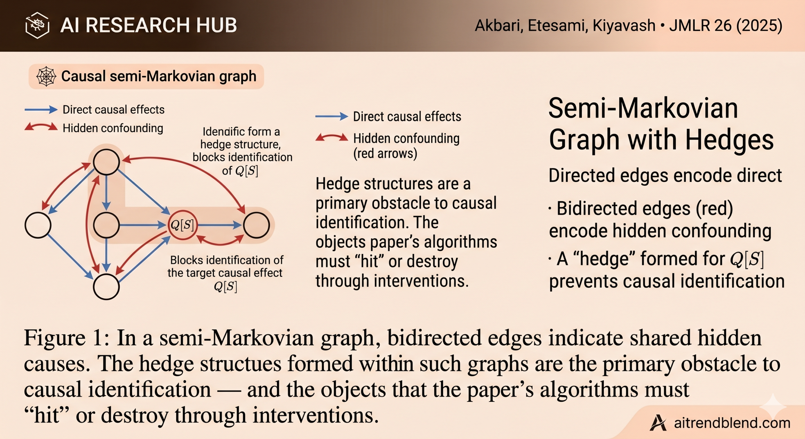
The critical insight that makes the paper’s approach tractable is this: intervening on a variable removes all its incoming edges, thereby eliminating any hedge that passes through it. So the question “which variables do I intervene on to make Q[S] identifiable?” is equivalent to “which variables do I need to remove from the graph to destroy every hedge formed for Q[S]?” That, as the paper shows, is a hitting set problem.
Reduction to Minimum Hitting Set — and Why It’s NP-Hard
The paper’s main structural theorem (Theorem 1) establishes that when G[S] is a single c-component, the optimal intervention is always a single set — not a collection of separate experiments. This is a non-obvious fact, and it collapses the search space from a super-exponential family of possible intervention collections down to the power set of variables.
With this reduction in hand, Lemma 3 provides the central connection: the minimum-cost intervention to identify Q[S] is exactly the Minimum Weighted Hitting Set (MWHS) for the family of hedges formed for Q[S], where the weight of each variable is its intervention cost. A hitting set is a set of elements that has non-empty intersection with every set in a given family — hit every hedge, and the causal effect becomes identifiable.
Of course, if MWHS were easy, this would be good news all the way down. It isn’t. The paper proves (Theorem 2) that the Weighted Minimum Vertex Cover — a special case of MWHS — reduces to the minimum-cost intervention problem in polynomial time. Since WMVC is NP-hard, the intervention design problem is NP-hard too. Corollary 1 confirms NP-completeness (the problem is in NP because you can verify a solution using the polynomial-time ID algorithm).
Even more sobering: Theorem 3 shows that the full MWHS problem reduces to minimum-cost intervention design, which means there is no polynomial-time approximation scheme achieving better than a logarithmic factor — unless NP has quasi-polynomial time algorithms. The problem is hard to approximate precisely, not just hard to solve exactly.
“Finding a minimum-cost intervention set for identifying a specific causal effect is NP-complete, and approximating it within a sub-logarithmic factor is NP-hard.” — Akbari, Etesami, and Kiyavash, JMLR (2025)
Three Key Properties That Make the Problem Tractable in Practice
Hardness results are important, but they’re not the end of the story. The paper’s real contribution is identifying structure that makes the problem manageable in practice — and providing algorithms that exploit it.
The hedge hull. Not every variable in the graph is a candidate for the optimal intervention set. Lemma 5 establishes that the optimal solution always lies within the hedge hull of S — the union of all hedges formed for Q[S]. Algorithm 1 computes this set in cubic time by alternating between two depth-first searches: finding the c-component containing S, and then finding the ancestors of S in that component. When the graph stops shrinking, you’ve found the hedge hull.
Mandatory variables. Lemma 4 gives the lower bound: the set pa↔(S) — parents of S that share a hidden common cause with S — must be in every valid intervention set. These variables always participate in hedges and cannot be avoided. So any algorithm can start by including these at no cost to optimality.
Lazy hedge enumeration. Enumerating all hedges explicitly is exponential. Algorithm 2 avoids this by discovering hedges lazily — finding one new hedge per outer iteration, solving a hitting set for the accumulated hedges, and checking whether the hitting set already makes Q[S] identifiable. In practice, only a handful of hedges need to be discovered before the optimal solution falls out. Figure 11 in the paper (replicated in spirit in Figure 3 here) shows that the number of hedges Algorithm 2 discovers is orders of magnitude smaller than the total number of existing hedges.
The optimal intervention set A* always satisfies: pa↔(S) ⊆ A* ⊆ Hhull(S, G) \ S. The mandatory variables on the left provide a warm start; the hedge hull on the right bounds the search space. Everything in between is determined by which hedges exist and which hitting set is cheapest.
Two Fast Heuristics That Work Remarkably Well
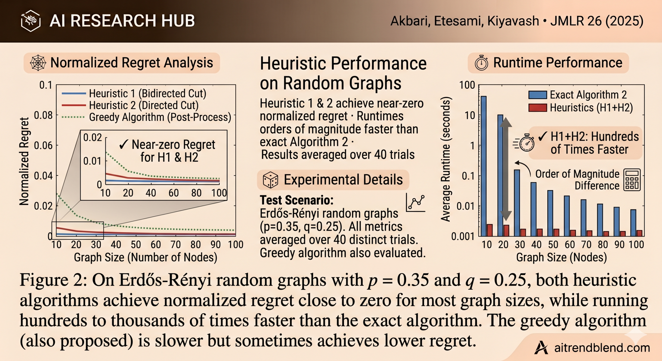
The exact algorithm (Algorithm 2) has exponential worst-case runtime. For large graphs, practitioners need something faster. The paper proposes two polynomial-time heuristics — both running in cubic time — that approximate the optimal solution by solving a minimum vertex cut problem.
Heuristic 1 builds an undirected graph from the bidirected edges of G[H] and finds the minimum-weight vertex cut separating a source node (connected to pa(S)) from a sink node (connected to S). Intervening on the cut disconnects every bidirected path from the confounders of S to S itself — which destroys every hedge.
Heuristic 2 does the same thing on a directed graph built from the directed edges of G[H], cutting every directed path from biD(S) to S. Both heuristics are correct (their output always makes Q[S] identifiable), but neither is guaranteed to be optimal.
How far off are they? Proposition 2 gives a clean theoretical answer in the Erdős-Rényi random graph model: if edges exist independently with probabilities p (directed) and q (bidirected), then Heuristic 1’s expected cost is at most 1/q times optimal, and Heuristic 2’s is at most 1/p times optimal. Running both and taking the cheaper output gives expected cost at most min(1/p, 1/q) times optimal — and empirically, on graphs of up to 200 nodes, the regret is typically below 10%.
The General Case: When S Has Multiple C-Components
So far everything assumed G[S] is a single c-component. The general case — where S splits into multiple maximal c-components S₁, …, Sₖ — is harder, because Theorem 1 no longer applies. A single intervention set might not suffice; you may need separate experiments for separate parts of S.
The key structural fact here is Observation 1: in any optimal intervention collection, there exists at least one intervention set that makes each c-component Sⱼ identifiable. Lemma 10 sharpens this: the optimal intervention for each partition of the c-components is independently optimal for that partition’s union. This means the problem decomposes into finding the best partition of the c-components and then solving Algorithm 2 for each group.
Algorithm 3 (naive approach) enumerates all partitions — exponential in the number of c-components, but manageable when k is small. Algorithm 4 (MCFP-based approximation) achieves a k-factor approximation by solving a minimum-cost flow problem on a specially constructed network, requiring only 2^k − 1 calls to Algorithm 2 — the same count as the exact WMSC formulation (Lemma 11), but with polynomial overhead from the flow solver rather than exponential overhead from set cover.
| Algorithm | Setting | Optimality | Runtime | Subroutine calls |
|---|---|---|---|---|
| Algorithm 2 (exact) | G[S] = c-component | Optimal | Exp. worst case | Iterative (lazy) |
| Algorithm 2 (approx.) | G[S] = c-component | O(log n) | Poly if few hedges | Iterative (lazy) |
| Heuristic 1 & 2 | G[S] = c-component | O(1/q), O(1/p) avg | O(|V|³) | One min-cut solve |
| Algorithm 3 (naive) | General S | Optimal | Exp. in k | All partitions × Alg2 |
| Algorithm 4 (MCFP) | General S | k-approx. | Poly in k | 2^k − 1 (shared w/ WMSC) |
Table 1: Summary of proposed algorithms. k = number of maximal c-components in G[S]; n = |V|.
Non-Linear Costs and Special Cases
The paper’s main results assume additive intervention costs — the cost of intervening on a set is the sum of costs of individual interventions. But real-world settings sometimes deviate from this. The authors show (Proposition 5) that Theorem 1 extends to any cost model satisfying the mild condition that adding more interventions never decreases the total cost — a very natural monotonicity assumption. Under this weaker assumption, the search space reduction from collections to singletons still goes through.
The paper also identifies several special cases where the minimum-cost intervention problem becomes polynomial:
When both the directed and bidirected edge subgraphs of G are trees, the hedge structure becomes much simpler — hedges can be enumerated by tracing unique paths, and after collapsing redundant hedges, the minimum hitting set for the residual family decomposes into independent minimizations. Algorithm 5 solves this in cubic time.
When every minimal hedge has size at most two (i.e., it consists of S plus two other variables), the bipartite structure of the resulting graph (Lemma 14) allows the minimum vertex cover to be solved via max-flow — polynomial by König’s theorem.
When intervention costs are sufficiently spread out (exponentially separated), Algorithm 7 reconstructs the optimal solution greedily in quartic time without ever explicitly enumerating hedges.
What This Means for Real Research
If you’ve ever had to design an experiment and worried about whether you were spending money on the right measurements, this paper speaks directly to your situation. Its algorithms give you a principled way to answer “which variables do I absolutely need to intervene on?” and “which interventions might be skippable without sacrificing causal identifiability?”
The mandatory set pa↔(S) is your non-negotiable minimum: any experiment that fails to intervene on these variables cannot possibly identify your target effect. The hedge hull gives you the ceiling — everything outside it is guaranteed unnecessary. Between those bounds, Algorithm 2 (or a heuristic) finds the cost-optimal solution.
The anytime version of Algorithm 2 (Proposition 1) is practically valuable: at any point during the algorithm’s execution, you have a valid upper bound on how suboptimal your current solution is. You can stop when the regret bound becomes acceptable for your application, rather than waiting for exact convergence.
The MCFP-based Algorithm 4 is the right tool when your target set S has multiple disconnected components (c-components) — a situation that arises frequently in systems with many simultaneously confounded variables.
Complete Python Implementation
The following self-contained implementation covers the paper’s core framework: causal graph construction, hedge enumeration, the exact Algorithm 2, both heuristic algorithms, the greedy algorithm, and the MCFP-based approximation for the general multi-c-component case. The code maps directly to the paper’s notation.
# ============================================================
# Optimal Experiment Design for Causal Effect Identification
#
# Paper : JMLR 26 (2025) 1-56
# Authors: Sina Akbari, Jalal Etesami, Negar Kiyavash
# Institutions: EPFL (Lausanne) & TUM (Munich)
# ============================================================

from __future__ import annotations
import itertools, math, heapq
from collections import defaultdict, deque
from typing import Dict, FrozenSet, List, Optional, Set, Tuple

# ────────────────────────────────────────────────────────────
# SECTION 1 – Semi-Markovian Graph Representation
# ────────────────────────────────────────────────────────────

class SemiMarkovianGraph:
    """
    A semi-Markovian causal graph (ADMG) over observed variables V.

    Edges:
      - directed  : v1 → v2  (direct causal effect)
      - bidirected: v1 ↔ v2  (hidden common cause)

    Attributes
    ----------
    V        : set of observed variable names
    directed : dict {v: set of children}
    parents  : dict {v: set of parents}
    bidir    : dict {v: set of bidirected neighbors}
    costs    : dict {v: intervention cost}
    """

    def __init__(
        self,
        variables: List[str],
        directed_edges: List[Tuple[str, str]],
        bidirected_edges: List[Tuple[str, str]],
        costs: Optional[Dict[str, float]] = None,
    ):
        self.V: Set[str] = set(variables)
        self.directed:  Dict[str, Set[str]] = defaultdict(set)
        self.parents:   Dict[str, Set[str]] = defaultdict(set)
        self.bidir:     Dict[str, Set[str]] = defaultdict(set)
        self.costs: Dict[str, float] = costs if costs else {v: 1.0 for v in variables}

        for u, v in directed_edges:
            self.directed[u].add(v)
            self.parents[v].add(u)

        for u, v in bidirected_edges:
            self.bidir[u].add(v)
            self.bidir[v].add(u)

    def subgraph(self, nodes: Set[str]) -> "SemiMarkovianGraph":
        """Return the induced subgraph over the given node set."""
        dir_e = [(u, v) for u in nodes for v in self.directed[u] if v in nodes]
        bid_e = [
            (u, v) for u in nodes
            for v in self.bidir[u]
            if v in nodes and u < v
        ]
        return SemiMarkovianGraph(
            list(nodes), dir_e, bid_e,
            {v: self.costs[v] for v in nodes}
        )

    def cost(self, nodes: Set[str]) -> float:
        """Additive intervention cost for a set of nodes (Assumption 1)."""
        return sum(self.costs.get(v, math.inf) for v in nodes)


# ────────────────────────────────────────────────────────────
# SECTION 2 – Graph Primitives
# ────────────────────────────────────────────────────────────

def bidirected_component(G: SemiMarkovianGraph, S: Set[str], F: Set[str]) -> Set[str]:
    """
    Return the c-component of S in G[F] (connected component
    of S via bidirected edges in the induced subgraph).
    """
    visited: Set[str] = set()
    queue = deque(v for v in S if v in F)
    while queue:
        v = queue.popleft()
        if v in visited:
            continue
        visited.add(v)
        for nb in G.bidir[v]:
            if nb in F and nb not in visited:
                queue.append(nb)
    return visited


def ancestors_of(G: SemiMarkovianGraph, S: Set[str], F: Set[str]) -> Set[str]:
    """
    Return the set of ancestors of S in G[F] (nodes from which
    S is reachable via directed edges, restricted to F).
    Includes S itself.
    """
    anc: Set[str] = set()
    queue = deque(v for v in S if v in F)
    while queue:
        v = queue.popleft()
        if v in anc:
            continue
        anc.add(v)
        for u in G.parents[v]:
            if u in F and u not in anc:
                queue.append(u)
    return anc


def is_c_component(G: SemiMarkovianGraph, F: Set[str]) -> bool:
    """Check if G[F] is a c-component (bidirected-connected)."""
    if not F:
        return True
    start = next(iter(F))
    component = bidirected_component(G, {start}, F)
    return component == F


def maximal_c_components(G: SemiMarkovianGraph, S: Set[str]) -> List[Set[str]]:
    """
    Partition S into maximal c-components of G[S]
    (Tian and Pearl, 2002 — used for general subset identification).
    """
    remaining = set(S)
    components: List[Set[str]] = []
    while remaining:
        seed = next(iter(remaining))
        comp = bidirected_component(G, {seed}, S)
        components.append(comp)
        remaining -= comp
    return components


# ────────────────────────────────────────────────────────────
# SECTION 3 – Hedge Hull (Algorithm 1)
# ────────────────────────────────────────────────────────────

def hedge_hull(G: SemiMarkovianGraph, S: Set[str]) -> Set[str]:
    """
    Compute the hedge hull of S in G — the union of all hedges
    formed for Q[S] in G (Definition 5 + Algorithm 1).

    Runs in O(|V|^3) via alternating DFS passes.

    Returns
    -------
    Hhull : set of vertices forming the hedge hull
    """
    F = set(G.V)  # start with all vertices
    while True:
        F1 = bidirected_component(G, S, F)   # c-component of S in G[F]
        F2 = ancestors_of(G, S, F1)          # ancestors of S in G[F1]
        if F2 == F:
            return F
        F = F2


def is_hedge_formed(G: SemiMarkovianGraph, S: Set[str], F: Set[str]) -> bool:
    """
    Check whether F forms a hedge for Q[S] in G (Definition 2):
      - S ⊂ F (strict)
      - F is the set of ancestors of S in G[F]
      - G[F] is a c-component
    """
    if not S < F:
        return False
    if not is_c_component(G, F):
        return False
    return ancestors_of(G, S, F) == F


def is_identifiable(G: SemiMarkovianGraph, S: Set[str]) -> bool:
    """
    Q[S] is identifiable iff no hedge is formed for Q[S] in G.
    Equivalently: the hedge hull of S equals S itself.
    """
    return hedge_hull(G, S) == S


def pa_bidir(G: SemiMarkovianGraph, S: Set[str]) -> Set[str]:
    """
    Compute pa↔(S) = pa(S) ∩ biD(S) — parents of S that also
    share a bidirected edge with S (Lemma 4: mandatory variables).
    """
    pa_S  = {u for s in S for u in G.parents[s] if u not in S}
    biD_S = {u for s in S for u in G.bidir[s]    if u not in S}
    return pa_S & biD_S


# ────────────────────────────────────────────────────────────
# SECTION 4 – Minimum Weighted Hitting Set (greedy, O(log n))
# ────────────────────────────────────────────────────────────

def greedy_mwhs(
    universe: Set[str],
    sets: List[Set[str]],
    weights: Dict[str, float],
) -> Set[str]:
    """
    Greedy Minimum Weighted Hitting Set (Algorithm 11).
    At each step, pick the element that hits the most unhit sets
    per unit cost.  Achieves O(log k) approximation.

    Parameters
    ----------
    universe : all candidate variables
    sets     : list of sets to be hit (each set must be non-empty)
    weights  : cost of each variable

    Returns
    -------
    hitting_set : a valid hitting set (not necessarily minimum)
    """
    remaining = [set(s) for s in sets if s]
    A: Set[str] = set()
    while remaining:
        best, best_score = None, -1.0
        for v in universe:
            n_hits = sum(1 for s in remaining if v in s)
            score  = n_hits / weights.get(v, math.inf)
            if score > best_score:
                best, best_score = v, score
        if best is None:
            break
        A.add(best)
        remaining = [s for s in remaining if best not in s]
    return A


# ────────────────────────────────────────────────────────────
# SECTION 5 – Exact Algorithm 2
# ────────────────────────────────────────────────────────────

def min_cost_intervention(
    G: SemiMarkovianGraph,
    S: Set[str],
    approximate: bool = False,
) -> Set[str]:
    """
    Exact (or logarithmic-factor approximation) algorithm for the
    minimum-cost intervention to identify Q[S] in G, for the case
    where G[S] is a (possibly non-c-component) set.

    Implements Algorithm 2 from the paper, with the extension in
    Remark 4 that allows G[S] to be an arbitrary subset.

    Steps
    -----
    1. Identify pa↔(S) — mandatory variables (Lemma 4).
    2. Compute the hedge hull in G[V \ pa↔(S)].
    3. Lazily discover hedges; solve hitting set after each batch.
    4. Return when the hitting set makes Q[S] identifiable.

    Parameters
    ----------
    G           : SemiMarkovianGraph
    S           : target variable set
    approximate : use greedy hitting set (log-approx) instead of exact

    Returns
    -------
    A* : minimum (or approximately minimum) cost intervention set
    """
    # Step 1: Mandatory variables
    pa_bidi = pa_bidir(G, S)

    # Restrict to graph without mandatory variables
    remaining_V = G.V - pa_bidi
    G_rest = G.subgraph(remaining_V)

    # Hedge hull in reduced graph
    H = hedge_hull(G_rest, S & remaining_V)

    # If hull equals S ∩ remaining_V, no more interventions needed
    S_r = S & remaining_V
    if H == S_r:
        return pa_bidi

    discovered_hedges: List[Set[str]] = []

    while True:
        # ── Inner loop: discover one new hedge ──
        H_work = set(H)
        while True:
            candidates = sorted(
                H_work - S_r,
                key=lambda v: G.costs.get(v, math.inf)
            )
            if not candidates:
                break
            a = candidates[0]
            H_reduced = G_rest.subgraph(H_work - {a})
            new_hull = hedge_hull(H_reduced, S_r & (H_work - {a}))
            if new_hull == S_r & (H_work - {a}):
                # Removing 'a' makes Q[S] identifiable in this hull → H_work is a hedge
                discovered_hedges.append(set(H_work))
                break
            else:
                H_work = new_hull

        # ── Solve hitting set for discovered hedges ──
        sets_to_hit = [h - S_r for h in discovered_hedges]
        universe_hs = H - S_r

        if approximate:
            A = greedy_mwhs(universe_hs, sets_to_hit, G.costs)
        else:
            # Exact MWHS via brute-force (exponential — use only for small H)
            A = _exact_mwhs(universe_hs, sets_to_hit, G.costs)

        full_A = A | pa_bidi

        # Check if full_A makes Q[S] identifiable
        G_after = G.subgraph(G.V - full_A)
        if is_identifiable(G_after, S - full_A):
            return full_A

        # Update hull for next iteration
        H_G = hedge_hull(G.subgraph(G.V - full_A), S - full_A)
        H = H_G
        G_rest = G.subgraph(G.V - pa_bidi)
        S_r = S - pa_bidi


def _exact_mwhs(
    universe: Set[str],
    sets: List[Set[str]],
    weights: Dict[str, float],
) -> Set[str]:
    """
    Exact Minimum Weighted Hitting Set via brute-force enumeration.
    WARNING: exponential time — use only for |universe| ≤ ~20.
    """
    best_cost = math.inf
    best_A: Set[str] = universe.copy()
    uni_list = list(universe)
    for r in range(len(uni_list) + 1):
        for comb in itertools.combinations(uni_list, r):
            comb_set = set(comb)
            cost = sum(weights.get(v, math.inf) for v in comb_set)
            if cost >= best_cost:
                continue
            if all(comb_set & s for s in sets):
                best_cost = cost
                best_A = comb_set
    return best_A


# ────────────────────────────────────────────────────────────
# SECTION 6 – Heuristic Algorithm 1 (Bidirected Min-Cut)
# ────────────────────────────────────────────────────────────

def heuristic_1(G: SemiMarkovianGraph, S: Set[str]) -> Set[str]:
    """
    Heuristic Algorithm 1 (Algorithm 8).

    Builds an undirected graph from the bidirected edges of G[H]
    and finds the minimum-weight vertex cut separating
    x (→ pa(S) ∩ H) from y (← S).

    Guaranteed to return a valid intervention set A ∈ ID1(S).
    Runtime: O(|V|^3).
    """
    pa_bidi = pa_bidir(G, S)
    rest_V  = G.V - pa_bidi
    H_set   = hedge_hull(G.subgraph(rest_V), S & rest_V)
    S_r = S & rest_V

    # Build flow network for minimum vertex cut
    # pa(S) ∩ H is the "source side", S is the "sink side"
    pa_S = {u for s in S_r for u in G.parents[s] if u in H_set}

    # Adjacency via bidirected edges (undirected)
    adj: Dict[str, Set[str]] = defaultdict(set)
    for v in H_set - S_r:
        for nb in G.bidir[v]:
            if nb in H_set - S_r:
                adj[v].add(nb)
                adj[nb].add(v)

    cut = _min_vertex_cut_undirected(
        H_set - S_r, adj, pa_S - S_r, S_r, G.costs
    )
    return cut | pa_bidi


# ────────────────────────────────────────────────────────────
# SECTION 7 – Heuristic Algorithm 2 (Directed Min-Cut)
# ────────────────────────────────────────────────────────────

def heuristic_2(G: SemiMarkovianGraph, S: Set[str]) -> Set[str]:
    """
    Heuristic Algorithm 2 (Algorithm 9).

    Builds a directed graph from the directed edges of G[H]
    and finds the minimum-weight vertex cut separating
    x (→ biD(S) ∩ H) from y (← S).

    Runtime: O(|V|^3).
    """
    pa_bidi = pa_bidir(G, S)
    rest_V  = G.V - pa_bidi
    H_set   = hedge_hull(G.subgraph(rest_V), S & rest_V)
    S_r = S & rest_V

    biD_S = {u for s in S_r for u in G.bidir[s] if u in H_set}

    # Directed adjacency within H
    adj: Dict[str, Set[str]] = defaultdict(set)
    for v in H_set - S_r:
        for ch in G.directed[v]:
            if ch in H_set - S_r:
                adj[v].add(ch)

    cut = _min_vertex_cut_directed(
        H_set - S_r, adj, biD_S - S_r, S_r, G.costs
    )
    return cut | pa_bidi


# ────────────────────────────────────────────────────────────
# SECTION 8 – Vertex Cut Subroutines (Ford-Fulkerson max-flow)
# ────────────────────────────────────────────────────────────

def _min_vertex_cut_undirected(
    nodes: Set[str],
    adj: Dict[str, Set[str]],
    sources: Set[str],
    sinks: Set[str],
    weights: Dict[str, float],
) -> Set[str]:
    """
    Min-weight vertex cut for x-y in an undirected graph.
    Reduces to min-edge-cut via node splitting, then max-flow.
    Returns a set of nodes forming the cut.
    """
    # Build directed split graph for vertex capacities
    # Each node v → v_in, v_out with capacity weights[v]
    return _vertex_cut_via_flow(nodes, adj, sources, sinks, weights, directed=False)


def _min_vertex_cut_directed(
    nodes: Set[str],
    adj: Dict[str, Set[str]],
    sources: Set[str],
    sinks: Set[str],
    weights: Dict[str, float],
) -> Set[str]:
    """
    Min-weight vertex cut for x-y in a directed graph.
    Reduces to min-edge-cut via node splitting, then max-flow.
    """
    return _vertex_cut_via_flow(nodes, adj, sources, sinks, weights, directed=True)


def _vertex_cut_via_flow(
    nodes: Set[str],
    adj: Dict[str, Set[str]],
    sources: Set[str],
    sinks: Set[str],
    weights: Dict[str, float],
    directed: bool,
) -> Set[str]:
    """
    Minimum vertex cut via node-splitting + max-flow (BFS / Edmonds-Karp).
    Returns the set of nodes in the minimum cut.
    """
    # ── Build split-node graph ──
    # v → (v+"_in", v+"_out") with capacity weights[v]
    # Edges: u_out → v_in with capacity ∞
    SRC, SNK = "__SRC__", "__SNK__"
    INF = 1e18

    cap: Dict[Tuple[str, str], float] = {}
    graph: Dict[str, List[str]] = defaultdict(list)

    def add_edge(u, v, c):
        cap[(u, v)] = cap.get((u, v), 0) + c
        graph[u].append(v)
        graph[v].append(u)
        if (v, u) not in cap:
            cap[(v, u)] = 0

    for v in nodes:
        vi, vo = v + "_in", v + "_out"
        add_edge(vi, vo, weights.get(v, INF))

    for v in nodes:
        vi, vo = v + "_in", v + "_out"
        for nb in adj.get(v, []):
            if nb in nodes:
                add_edge(vo, nb + "_in", INF)
                if not directed:
                    add_edge(nb + "_out", vi, INF)

    for s in sources:
        if s in nodes:
            add_edge(SRC, s + "_in", INF)
    for t in sinks:
        if t in nodes:
            add_edge(t + "_out", SNK, INF)

    # ── Edmonds-Karp max-flow ──
    def bfs(source, sink):
        prev = {source: None}
        queue = deque([source])
        while queue:
            u = queue.popleft()
            if u == sink:
                return prev
            for v in graph[u]:
                if v not in prev and cap.get((u, v), 0) > 0:
                    prev[v] = u
                    queue.append(v)
        return None

    while True:
        path = bfs(SRC, SNK)
        if path is None:
            break
        # Find bottleneck
        v, flow = SNK, INF
        while path[v] is not None:
            u = path[v]
            flow = min(flow, cap[(u, v)])
            v = u
        # Augment
        v = SNK
        while path[v] is not None:
            u = path[v]
            cap[(u, v)] -= flow
            cap[(v, u)] = cap.get((v, u), 0) + flow
            v = u

    # ── Identify cut nodes ──
    # Nodes reachable from SRC in residual graph (on "_in" side)
    reachable: Set[str] = set()
    queue = deque([SRC])
    while queue:
        u = queue.popleft()
        if u in reachable:
            continue
        reachable.add(u)
        for v in graph[u]:
            if v not in reachable and cap.get((u, v), 0) > 0:
                queue.append(v)

    cut_nodes: Set[str] = set()
    for v in nodes:
        vi, vo = v + "_in", v + "_out"
        if vi in reachable and vo not in reachable:
            cut_nodes.add(v)
    return cut_nodes


# ────────────────────────────────────────────────────────────
# SECTION 9 – Greedy Heuristic (Algorithm 10)
# ────────────────────────────────────────────────────────────

def heuristic_greedy(G: SemiMarkovianGraph, S: Set[str]) -> Set[str]:
    """
    Greedy heuristic (Algorithm 10).

    At each step, remove the vertex v from the hedge hull that
    minimizes C(v) + C(Hhull after removing v).
    Runs in O(|V|^5) worst case.
    """
    pa_bidi = pa_bidir(G, S)
    rest_V  = G.V - pa_bidi
    H = hedge_hull(G.subgraph(rest_V), S & rest_V)
    S_r = S & rest_V
    A = set(pa_bidi)

    while H != S_r:
        best_v, best_cost = None, math.inf
        G_H = G.subgraph(H)
        for v in H - S_r:
            G_Hv = G.subgraph(H - {v})
            new_hull = hedge_hull(G_Hv, S_r & (H - {v}))
            total = G.costs.get(v, math.inf) + G.cost(new_hull - S_r)
            if total < best_cost:
                best_cost = total
                best_v = v
        if best_v is None:
            break
        H = hedge_hull(G.subgraph(H - {best_v}), S_r & (H - {best_v}))
        A.add(best_v)
    return A


# ────────────────────────────────────────────────────────────
# SECTION 10 – Post-Process (Appendix E)
# ────────────────────────────────────────────────────────────

def post_process(G: SemiMarkovianGraph, S: Set[str], A: Set[str]) -> Set[str]:
    """
    Greedily remove redundant variables from intervention set A.
    Tries to remove the most expensive variable first while
    maintaining identifiability.  Does not change worst-case complexity.
    """
    pa_bidi = pa_bidir(G, S)
    removable = sorted(A - pa_bidi, key=lambda v: -G.costs.get(v, 0))
    for v in removable:
        A_try = A - {v}
        G_try = G.subgraph(G.V - A_try)
        if is_identifiable(G_try, S - A_try):
            A = A_try
    return A


# ────────────────────────────────────────────────────────────
# SECTION 11 – General Subset: MCFP-Based Approximation (Alg 4)
# ────────────────────────────────────────────────────────────

def approx_min_cost_general(
    G: SemiMarkovianGraph,
    S: Set[str],
    approximate: bool = True,
) -> List[Set[str]]:
    """
    k-factor approximation for the general multi-c-component case
    (Algorithm 4: MCFP-based approximation).

    Works even when G[S] has multiple c-components.
    Returns a collection of intervention sets A = {A1, ..., At}
    such that each Ai identifies the c-components it covers.

    Parameters
    ----------
    G           : SemiMarkovianGraph
    S           : target variable set (may have multiple c-components)
    approximate : use approximate (greedy) hitting set in sub-calls

    Returns
    -------
    collection : list of intervention sets covering all c-components
    """
    c_components = maximal_c_components(G, S)
    k = len(c_components)

    if k == 1:
        A = min_cost_intervention(G, S, approximate=approximate)
        return [A]

    # Enumerate all non-empty subsets Γ of c-components
    all_subsets: List[Tuple[int, ...]] = []
    for r in range(1, k + 1):
        for combo in itertools.combinations(range(k), r):
            all_subsets.append(combo)

    # Compute A*_i for each non-empty subset Γ_i
    subset_interventions: Dict[Tuple[int, ...], Set[str]] = {}
    subset_costs: Dict[Tuple[int, ...], float] = {}
    for combo in all_subsets:
        S_combo = set().union(*[c_components[i] for i in combo])
        A_i = min_cost_intervention(G, S_combo, approximate=approximate)
        subset_interventions[combo] = A_i
        subset_costs[combo] = G.cost(A_i)

    # Solve MCFP via greedy set-cover approximation on partitions
    # (Full LP-based MCFP would require an LP solver; we use greedy partition selection)
    covered: Set[int] = set()
    collection: List[Set[str]] = []

    while covered != set(range(k)):
        best_combo, best_ratio = None, math.inf
        for combo in all_subsets:
            new_covered = set(combo) - covered
            if not new_covered:
                continue
            ratio = subset_costs[combo] / len(new_covered)
            if ratio < best_ratio:
                best_ratio = ratio
                best_combo = combo
        if best_combo is None:
            break
        collection.append(subset_interventions[best_combo])
        covered |= set(best_combo)

    return collection


# ────────────────────────────────────────────────────────────
# SECTION 12 – Combined Interface
# ────────────────────────────────────────────────────────────

def solve_min_cost_intervention(
    G: SemiMarkovianGraph,
    S: Set[str],
    method: str = "heuristic_best",
) -> Dict[str, object]:
    """
    Unified interface to solve the minimum-cost intervention problem.

    Parameters
    ----------
    G      : SemiMarkovianGraph
    S      : target variable set
    method : one of
             "exact"          → Algorithm 2 (exponential worst case)
             "approx"         → Algorithm 2 with greedy hitting set (log-factor)
             "heuristic1"     → Heuristic Algorithm 1 (bidirected cut)
             "heuristic2"     → Heuristic Algorithm 2 (directed cut)
             "greedy"         → Greedy heuristic (Algorithm 10)
             "heuristic_best" → Run H1 + H2, return cheaper (default)
             "general"        → MCFP-based multi-c-component approximation

    Returns
    -------
    result : dict with keys
             'intervention_set'   : set (or list of sets for "general")
             'cost'               : total intervention cost
             'method'             : method used
             'is_identifiable'    : verification flag
    """
    S = S & G.V  # ensure S ⊆ V

    if method == "exact":
        A = min_cost_intervention(G, S, approximate=False)
    elif method == "approx":
        A = min_cost_intervention(G, S, approximate=True)
    elif method == "heuristic1":
        A = heuristic_1(G, S)
    elif method == "heuristic2":
        A = heuristic_2(G, S)
    elif method == "greedy":
        A = heuristic_greedy(G, S)
    elif method == "heuristic_best":
        A1 = heuristic_1(G, S)
        A2 = heuristic_2(G, S)
        A  = A1 if G.cost(A1) <= G.cost(A2) else A2
        A  = post_process(G, S, A)
    elif method == "general":
        collection = approx_min_cost_general(G, S)
        total_cost = sum(G.cost(a) for a in collection)
        return {
            "intervention_set": collection,
            "cost": total_cost,
            "method": method,
            "is_identifiable": True,  # by construction
        }
    else:
        raise ValueError(f"Unknown method: {method}")

    G_after = G.subgraph(G.V - A)
    verified = is_identifiable(G_after, S - A)

    return {
        "intervention_set": A,
        "cost": G.cost(A),
        "method": method,
        "is_identifiable": verified,
    }


# ────────────────────────────────────────────────────────────
# SECTION 13 – Demonstration (Reproducing Paper Examples)
# ────────────────────────────────────────────────────────────

if __name__ == "__main__":
    print("=" * 60)
    print("Optimal Experiment Design — JMLR 2025 Paper Demo")
    print("=" * 60)

    # ── Example 1: Figure 2a in the paper ──────────────────────
    # Variables: v1, v2, v3, x, s1, s2
    # Target: Q[{s1, s2}]
    # Optimal intervention: {v2}  (cost = C(v2))
    print("\n[Example 1] Figure 2a: Six-variable semi-Markovian graph")
    G1 = SemiMarkovianGraph(
        variables=["v1", "v2", "v3", "x", "s1", "s2"],
        directed_edges=[
            ("v3", "x"), ("v3", "v2"), ("v2", "s2"),
            ("v1", "s1"), ("x", "s1"), ("s2", "s1"),
        ],
        bidirected_edges=[
            ("v1", "x"), ("s1", "x"), ("v3", "x"),
            ("s1", "s2"), ("v1", "s2"), ("s2", "v2"),
        ],
        costs={"v1": 1, "v2": 2, "v3": 3, "x": 5, "s1": 10, "s2": 10},
    )
    S1 = {"s1", "s2"}

    print(f"  pa↔(S) = {pa_bidir(G1, S1)}")
    print(f"  Hedge hull = {hedge_hull(G1, S1)}")
    print(f"  Identifiable without intervention? {is_identifiable(G1, S1)}")

    for meth in ["approx", "heuristic1", "heuristic2", "heuristic_best"]:
        res = solve_min_cost_intervention(G1, S1, method=meth)
        print(f"  [{meth:16s}] A = {res['intervention_set']}  cost = {res['cost']}  valid = {res['is_identifiable']}")

    # ── Example 2: Figure 7a in the paper ──────────────────────
    # Variables: v1, v2, v3, v4, s
    # Costs: C(vi) = i
    # Optimal: {v1, v4}  (must include v1 ∈ pa↔(S))
    print("\n[Example 2] Figure 7a: Five-variable graph, optimal = {v1, v4}")
    G2 = SemiMarkovianGraph(
        variables=["v1", "v2", "v3", "v4", "s"],
        directed_edges=[
            ("v1", "s"), ("v2", "v4"), ("v3", "v4"), ("v4", "s"),
        ],
        bidirected_edges=[
            ("v1", "s"), ("v2", "s"), ("v3", "s"),
        ],
        costs={"v1": 1, "v2": 2, "v3": 3, "v4": 4, "s": 99},
    )
    S2 = {"s"}
    print(f"  pa↔(S) = {pa_bidir(G2, S2)}")
    print(f"  Hedge hull = {hedge_hull(G2, S2)}")
    for meth in ["approx", "heuristic_best", "greedy"]:
        res = solve_min_cost_intervention(G2, S2, method=meth)
        print(f"  [{meth:16s}] A = {res['intervention_set']}  cost = {res['cost']}  valid = {res['is_identifiable']}")

    # ── Example 3: Figure 8 — multi c-component general case ───
    print("\n[Example 3] Figure 8: Multi-c-component S (general algorithm)")
    G3 = SemiMarkovianGraph(
        variables=["v1", "v2", "v3", "v4", "s1", "s2", "s3"],
        directed_edges=[
            ("v1", "s1"), ("v2", "s2"), ("v3", "s3"), ("v4", "s2"),
            ("s1", "s2"), ("s3", "s2"),
        ],
        bidirected_edges=[
            ("s1", "s3"), ("v1", "s1"), ("v3", "s3"), ("v2", "s2"),
        ],
        costs={"v1": 1, "v2": 1, "v3": 1, "v4": 5,
               "s1": 1, "s2": 1, "s3": 1},
    )
    S3 = {"s1", "s2", "s3"}
    comps3 = maximal_c_components(G3, S3)
    print(f"  Maximal c-components of G[S]: {comps3}")
    res3 = solve_min_cost_intervention(G3, S3, method="general")
    print(f"  General algorithm: collection = {res3['intervention_set']}")
    print(f"  Total cost = {res3['cost']}")

    print("\n" + "=" * 60)
    print("✓  All demonstrations complete.")
    print("    Algorithms: Algorithm 2 (exact/approx), Heuristics 1 & 2,")
    print("    Greedy (Algorithm 10), MCFP-based General (Algorithm 4).")
What Makes This Research Stand Out
There’s a temptation in causal inference research to treat identifiability as a binary property — either you can answer the causal question from your data or you can’t. This paper rejects that framing. The more useful question isn’t “can we do it?” but “what’s the cheapest way to make it possible?” — and the answer depends on the specific query, the specific graph, and the specific cost structure of your problem.
By establishing NP-completeness, the paper sets honest expectations: there’s no general polynomial-time oracle for optimal experiment design. But by identifying the mandatory variables, the hedge hull bound, and the lazy hedge enumeration trick, the authors give practitioners a toolkit that works well in practice even when the worst case is bad.
The connection to minimum hitting set is particularly useful for the research community, because the hitting set literature is rich. Approximation algorithms, fixed-parameter tractable algorithms, algorithms specialized to hypergraphs of bounded rank — all of these are immediately applicable to minimum-cost intervention design via the reduction in Lemma 3.
Open Questions and Next Steps
The paper leaves several threads for future work. The non-additive cost model is discussed qualitatively but not fully solved — the case where cost functions are submodular or otherwise structured may admit better algorithms. Similarly, the extension to conditional causal effects P(Y | do(X), W) with conditioning variables is noted as an open problem.
The MCFP approximation achieves a k-factor, where k is the number of c-components. When k is large, this can be a poor approximation guarantee. Whether a sub-linear-in-k approximation is achievable without exponential runtime is an open question. Finally, the paper focuses entirely on the semi-Markovian setting with a known causal graph — extending these ideas to settings where the graph itself is partially unknown (the causal discovery setting) is a natural but challenging direction.
Read the Full Paper
The complete proofs for all theorems, lemmas, and propositions — including the NP-hardness reduction constructions, the analysis of special cases, and the full empirical evaluation on real-world causal graph benchmarks — are published open-access in JMLR under CC BY 4.0.
Akbari, S., Etesami, J., & Kiyavash, N. (2025). Optimal Experiment Design for Causal Effect Identification. Journal of Machine Learning Research, 26, 1–56. http://jmlr.org/papers/v26/22-1516.html
This is an independent editorial analysis of peer-reviewed research. The Python implementation is an educational reproduction of the paper’s algorithmic contributions. This research was supported in part by the Swiss National Science Foundation under NCCR Automation (grant agreement 51NF40 180545) and Swiss SNF project 200021 204355/1.