Key points
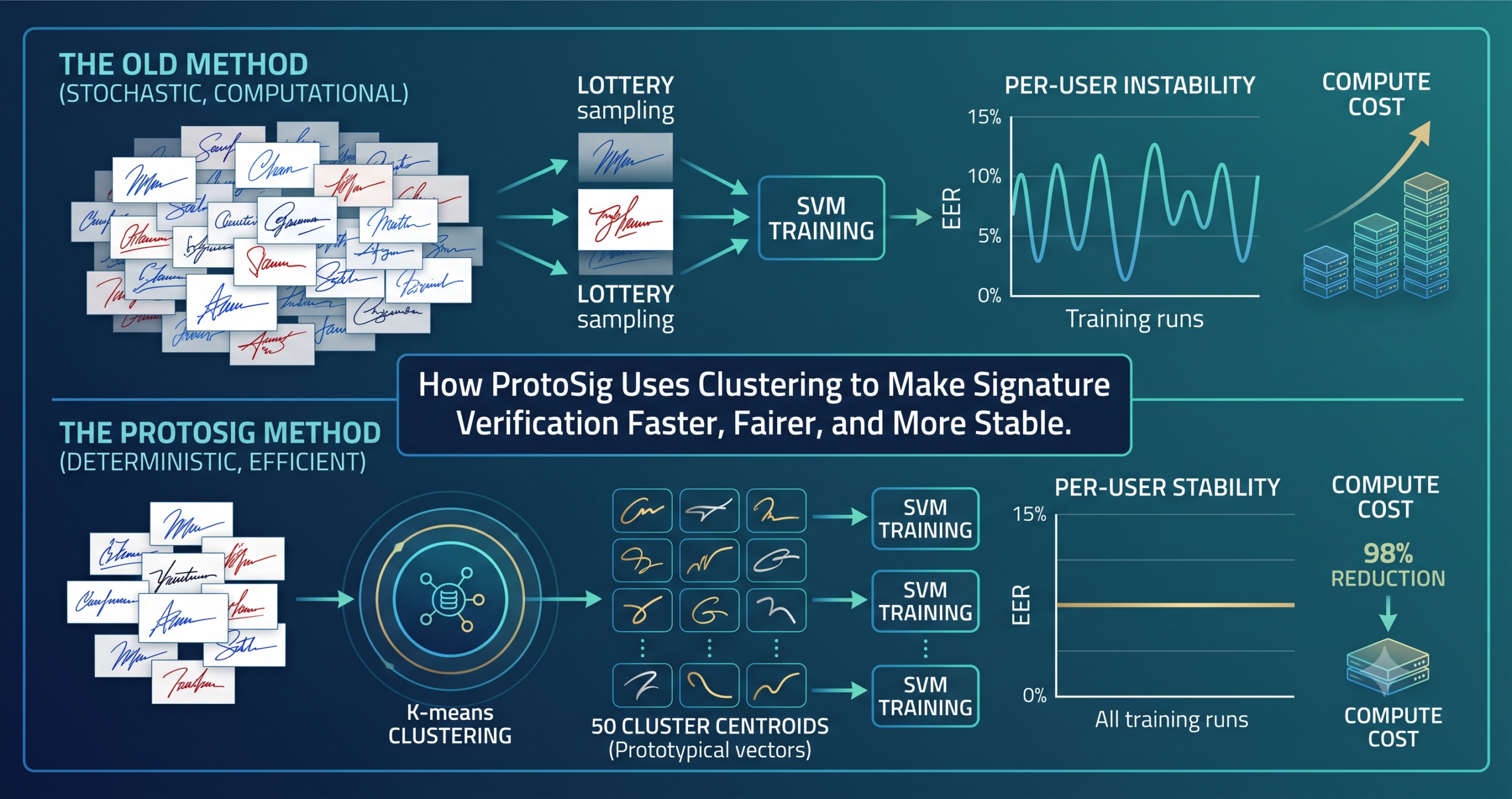
- ProtoSig replaces the standard practice of randomly sampling other users’ signatures as negative training examples with a small set of cluster centroids that represent the overall signature distribution, reducing the negative training set from thousands of samples to 50.
- The method runs K-means clustering once on a combined development dataset to produce non-identifiable prototypical signature vectors, which are then reused across all users without accessing external biometric data again.
- On GPDS Synthetic at maximum scale, training time drops from 97 seconds to just over 1 second, and training FLOPs fall by approximately two orders of magnitude, while verification accuracy matches or exceeds the standard approach.
- The EER for individual users in a writer dependent system can vary by more than 20 percentage points across runs under standard random sampling. ProtoSig eliminates this variability entirely, since every training run draws the same fixed set of prototypes.
- Gini coefficient analysis shows the standard approach’s false accept errors concentrate systematically on specific attackers (GC 0.81), while ProtoSig distributes those errors essentially at random across the attacker population (GC 0.48), which is the fairer outcome for deployment.
- The prototypical vectors are cluster centroids mixing hundreds of users’ signatures, which makes re-identification substantially harder. Silhouette scores drop from 0.22 to 0.04 after summarization, and cluster purity averages just 0.09 across the GPDS Synthetic dataset.
The random forgery problem and why nobody measured its instability
Offline handwritten signature verification systems face a fundamental data problem. Real forgery examples are almost never available during training, because collecting them requires skilled impostors to practice copying specific people’s signatures, which does not happen naturally in the datasets available to researchers. The standard workaround is to treat genuine signatures from other users in the dataset as stand-ins for forgeries, under the assumption that the classifier will learn to reject anything that does not belong to the user it was trained for. These stand-ins are called random forgeries in the literature, and every major HSV system reviewed in this paper uses them.
The random forgery approach has a number of well-understood weaknesses. The randomly chosen samples may not be the most informative negatives for training a good decision boundary. Using thousands of other users’ signatures introduces storage and compute costs that scale linearly with the number of enrolled users. And accessing raw biometric data from external users raises privacy concerns that complicate deployment, particularly in jurisdictions where biometric storage is regulated.
What the paper identifies as a previously unstudied problem is the stochastic instability this sampling introduces at the individual user level. In a writer dependent system, each enrolled user gets their own classifier trained fresh whenever the system is updated. The negative samples drawn for that training run are chosen at random from the pool of other users’ signatures. Different draws produce different classifiers, and because the draws are random, the performance for any given user can vary substantially from one training run to the next. The paper formalizes this by repeating the same experiment five times, keeping the genuine training signatures fixed and varying only which negatives were sampled, and reports that individual user EERs varied by more than 20 percentage points across those five runs.
This is a genuine deployment risk. A security system that behaves predictably for most users but unpredictably for a subset, depending on when its models happen to be retrained, gives administrators no reliable way to audit or audit-trail the system’s behavior per user. The paper is, to the authors’ knowledge, the first to formally study and quantify this instability in the HSV literature.
The ProtoSig approach, clustering as a substitute for random sampling
The core idea in ProtoSig is elegant. Rather than selecting negative training samples by random draw from a pool of thousands of other users’ raw signatures, the method first summarizes that entire pool into a small set of representative vectors. Those vectors become the fixed negative samples used for every user’s classifier on every training run.
The summarization step runs clustering on the full development dataset’s feature vectors. The method is agnostic about which clustering algorithm is used, and the paper experiments with K-means, Gaussian Mixture Models, agglomerative hierarchical clustering, BIRCH, DBSCAN, and unsupervised dictionary learning to validate this agnosticism. Because clustering partitions the feature space into regions based on similarity across the entire population of users, the resulting cluster centroids naturally aggregate characteristics from many different writers rather than representing any single one. That mixing is both the source of their informativeness as training negatives and the source of their privacy protection as stored vectors.
The prototypical signatures produced by this step are feature space vectors, not images. They are not reconstructions of any user’s actual handwriting. They are mathematical summaries of the shape of the distribution. Once generated, they can be stored as a compact set of numbers and reused across every writer dependent classifier in the system without any further access to the original biometric data.
The training set construction for each user follows a straightforward formula. The genuine feature vectors from the target user form the positive class, and the full set of k prototypical signatures forms the negative class.
Where \(\mathcal{X}_j\) is the set of genuine feature vectors for user j, and \(\mathcal{C} = \{\mathbf{c}_1, \ldots, \mathbf{c}_k\}\) is the fixed set of prototypical signatures. Every user gets the same negative class, and no per-user selection or distance computation is needed. The whole point of the summarization step is that \(\mathcal{C}\) already captures the distribution of the feature space comprehensively enough that random selection becomes unnecessary.
Experimental setup
The paper tests ProtoSig across three public datasets with meaningfully different characteristics. CEDAR, a smaller dataset with 55 subjects each providing 24 genuine and 24 skilled forgery signatures. MCYT-75, a mid-sized dataset with 75 subjects at 15 signatures each. And GPDS Synthetic, a large-scale dataset with 10,000 subjects and 24 genuine plus 30 skilled forgery signatures each, which is where the computational comparisons are most dramatic.
Feature extraction uses SigNet-S, a deep CNN producing 2048-dimensional feature vectors, trained on a disjoint user subset of GPDS Synthetic to ensure no leakage into the experimental data. Classification uses an SVM-RBF classifier from scikit-learn with C equal to 1.0 and kernel coefficient γ equal to 2 to the power of negative 11, following established practice in the literature. Performance is measured with EER at both global and user-specific thresholds, repeated five times, and reported as mean plus or minus standard deviation.
The two baselines are the leave one out approach, which draws negatives from all other users in the development set (reaching 3,588 negative samples for GPDS Synthetic at maximum training signatures), and a multi-dataset configuration that pools all three development sets and draws randomly from the combined pool of 645 samples. ProtoSig uses k equal to 50 prototypical signatures across all comparisons, selected via cross-validation.
Results on verification accuracy
Across all three datasets and all training set sizes from one to twelve genuine signatures per user, ProtoSig matches or exceeds both baselines on EER. The improvement is not always large, but it is consistent, and it is achieved with dramatically fewer negative samples. Figure 8 in the paper visualizes this directly: the LOO curve requires more than 3,500 negative samples and reaches EER around 3.1% on GPDS Synthetic with user-specific thresholds, while ProtoSig achieves a similar EER at a single fixed point of 50 samples. The full detail on training configurations from Table 5 shows that for GPDS Synthetic at twelve genuine signatures per user, K-means, GMM, and agglomerative clustering all reach mean EER around 5.6% to 5.7% at global thresholds, very close to what the leave one out baseline achieves with 71 times as many negative samples.
The Friedman statistical test across all clustering methods except dictionary learning found no significant performance differences at the 5% level. The p-value was 0.058 under global thresholds and 0.070 under user-specific thresholds. The practical interpretation is that ProtoSig’s performance gains come from the summarization principle rather than from any particular choice of clustering algorithm. K-means was adopted for the subsequent experiments because it achieved the best average ranking, but any of the other algorithms (except dictionary learning, which failed because it is designed for sparse signal reconstruction rather than data partitioning) would work nearly as well.
Computational cost, the numbers that change the deployment conversation
| Metric | Standard (LOO) | ProtoSig (k=50) |
|---|---|---|
| Training time (seconds) | 97.39 | 1.01 |
| Training FLOPs | 3.46 × 10¹¹ | 5.08 × 10⁹ |
| Testing time (seconds) | 0.80 | 0.68 |
| Testing FLOPs | 3.98 × 10⁹ | 3.26 × 10⁹ |
| Number of support vectors | 21,362 | 17,498 |
| Model size (KB) | 348,856 | 288,401 |
The training time reduction from 97 seconds to just over 1 second is the headline number. But the FLOPs comparison tells the more structural story. Standard sampling at this scale requires 3.46×10¹¹ floating point operations during training. ProtoSig requires 5.08×10⁹, roughly two orders of magnitude less. At smaller scales the absolute savings are smaller, but the scaling curve is the important thing. Standard sampling’s compute cost grows linearly as the number of enrolled users grows, because each new user’s classifier needs to be trained on more negative samples drawn from all others. ProtoSig’s cost is essentially flat, because the negative set stays at 50 regardless of how many users join the system.
Stability, the result that changes what deployment actually looks like
The paper makes the case for stability with a careful experiment. The genuine training signatures for each user are held fixed across five runs. Only the negative samples change between runs, drawn fresh from the development set each time. Then the EER is computed per user after each run, and the variation across the five runs is recorded. Under standard sampling, the average EER range per user can exceed several percentage points even at the largest development set sizes. And for individual users, the swings are much larger. User 12 in the full 581-user configuration showed EERs of 5%, 5%, 5%, 15%, and 5% across five runs. User 209 showed 5%, 15%, 10%, 10%, and 10%. These are not edge cases selected for drama. They are the four worst-performing users presented as examples of a systematic phenomenon.
Under ProtoSig, the EER variation across all runs for all users is negligibly small, essentially zero. That is not surprising: the negative samples are the same every time. What is notable is that fixing the negatives to the same 50 cluster centroids does not introduce a new bias that hurts average performance. The stable result is also the accurate result.
“The EER for some users varied by more than 20 percentage points across different runs.” Kecia G. de Moura et al., École de technologie supérieure, Pattern Recognition 2026
Fairness, what the Gini coefficient reveals about error distribution
Beyond per-user stability, the paper uses Lorenz curves and Gini coefficients to assess whether errors are distributed equitably across users. The motivation comes from the biometric fairness literature: a system where all false accepts go to the same subset of attackers gives those specific attackers a persistent advantage over the detection system, which is a security property distinct from the overall error rate.
Under standard sampling, the Gini coefficient for false acceptance rate across attackers was 0.81 on GPDS Synthetic, indicating that a small fraction of attackers accounted for a disproportionate share of successful bypass events. This is the pattern of systematic error, where the same people reliably fool the system. Under ProtoSig, the corresponding Gini coefficient was 0.48, much closer to the value that would indicate errors distributed uniformly at random across the attacker population.
For false rejections, the interpretation reverses. A higher Gini coefficient for FRR is actually preferable, because it means that false rejections are concentrated among a few users rather than distributed evenly, which in practice means those few users’ situations can be identified and addressed through calibration or additional authentication channels. Standard sampling gives a FRR Gini coefficient of 0.72. ProtoSig gives 0.98, suggesting that under ProtoSig, false rejections are concentrated in a small, identifiable group of outlier users whose signing behavior may be erratic or whose enrollment data was poor, which is operationally actionable. A large, uniform distribution of false rejections across many users is harder to triage.
Privacy analysis, what the cluster centroids actually reveal
Storing biometric templates raises the question of whether those templates can be used to reconstruct the original biometric data. This concern is formalized in the inverse biometrics literature, and the paper addresses it directly by measuring how much identifiable information survives the summarization step.
Two metrics capture this. Cluster purity measures what fraction of signatures in each cluster come from the same user. High purity would mean a given prototypical vector is basically a signature for a specific person, which would be a privacy problem. Low purity means signatures from many different writers got mixed into each cluster. At k equal to 50 on GPDS Synthetic, the average cluster purity was 0.09, meaning each cluster contains signatures from many users with no single writer dominating. Cluster entropy reached 0.85 out of a normalized maximum of 1, indicating close to uniform mixing of writers within clusters.
The silhouette coefficient measures how distinctly clustered different users’ signatures remain after the summarization. A high silhouette score would mean writer-specific clusters are still well-separated after ProtoSig, which would make re-identification easier. The silhouette coefficient dropped from 0.22 on the original feature vectors (before summarization) to 0.04 on the prototypical vectors, indicating that the original per-writer cluster structure has been substantially dissolved. Different writers’ data overlaps heavily in the post-summarization representation.
Plug-in evaluation with published systems
The strongest practical claim in the paper is that ProtoSig can be dropped into any existing writer dependent HSV system that uses random forgeries as negatives, and the result will be statistically equivalent performance at lower cost. The paper tests this by integrating ProtoSig into two recent published systems for which reproducible code was available.
The first is the feature knowledge distillation approach from Tsourounis et al. 2025, which trains a ResNet-18 student model using three knowledge distillation strategies (GEOM and TCE, GEOM and BT, and GEOM and BC) from a SigNet teacher, without requiring signature images during distillation. The second is the continual learning approach from Viana et al. 2024, which distills knowledge from a SigNet teacher into student models across three architectures: Continual SigNet (AlexNet based), Continual ResNet152, and Continual Vision Transformer.
For each of these six backbone configurations across multiple datasets, the paper reports EER with and without ProtoSig, along with p-values from paired statistical tests and Bayesian ROPE analysis. The Region of Practical Equivalence used was ±0.015, reflecting the judgment that differences smaller than 1.5 percentage points in EER are not practically meaningful. In the large majority of configurations, over 95% of the posterior probability of the EER difference fell within the ROPE, confirming statistical equivalence. There are a handful of cases, specifically Continual SigNet and Continual ViT on the SGPDS datasets with user-specific thresholds, where the p-value is significant and the HDI falls slightly outside the ROPE on the upper end, suggesting ProtoSig does impose a small but measurable cost on those configurations. The paper does not dismiss these cases and the Bayesian analysis treats them as what they are: small but non-negligible differences in a subset of configurations.
Limitations the paper states honestly
- All experiments use deep CNN features. Whether ProtoSig provides the same benefits with handcrafted feature representations was not assessed, and different feature types might respond differently to the summarization approach.
- The privacy evaluation relies on indirect distributional measures, silhouette scores, purity, and entropy. No adversarial re-identification attack was run against the stored prototypical vectors, so no formal privacy guarantee can be claimed.
- ProtoSig is evaluated in writer dependent settings. The extension to writer independent verification, where a single shared model handles all users, is described as a natural direction but was not experimentally validated in this work.
- Presentation attack detection (detecting physical spoofs such as printed signatures or screen captures) is outside the scope of ProtoSig, which is a training data strategy rather than a detection method.
- The Bayesian ROPE analysis found a small number of configurations where the EER difference fell slightly outside the region of practical equivalence, particularly with continual learning backbones on larger GPDS subsets under user-specific thresholds.
A reference implementation
The code below is an independent educational implementation of the ProtoSig pipeline. It combines a simplified SigNet-style CNN in PyTorch for feature extraction with the K-means summarization and SVM-RBF classification stages from the paper. The full paper is available at the Pattern Recognition journal. This implementation uses synthetic dummy data for the smoke test rather than real signature images.
# protosig_reference.py
# Independent educational implementation of the ProtoSig pipeline.
# Source paper: de Moura, Sabourin, Cruz. ProtoSig.
# Pattern Recognition 180 (2026) 114258. DOI 10.1016/j.patcog.2026.114258
# Not the authors' released code. Written from the method description only.

import numpy as np
import torch
import torch.nn as nn
import torch.nn.functional as F
from sklearn.cluster import KMeans
from sklearn.svm import SVC
from sklearn.metrics import silhouette_score
from sklearn.preprocessing import normalize
from scipy.stats import entropy as scipy_entropy


# ──────────────────────────────────────────────────────────────────────────────
# Feature extractor: SigNet-style deep CNN
# Paper uses SigNet Synthetic (SigNet-S), a CNN producing 2048-dim vectors.
# We implement a simplified version for educational purposes.
# ──────────────────────────────────────────────────────────────────────────────

class SigNetLike(nn.Module):
    """Simplified SigNet-style CNN feature extractor.

    The real SigNet-S (Viana et al. 2023) produces 2048-dim vectors from
    signature images resized to 150x220 pixels. This simplified version
    demonstrates the architecture concept on smaller inputs.
    """

    def __init__(self, output_dim=2048):
        super().__init__()
        self.features = nn.Sequential(
            nn.Conv2d(1, 32, kernel_size=5, stride=2, padding=2),
            nn.BatchNorm2d(32),
            nn.ReLU(inplace=True),
            nn.MaxPool2d(2),

            nn.Conv2d(32, 64, kernel_size=3, padding=1),
            nn.BatchNorm2d(64),
            nn.ReLU(inplace=True),
            nn.MaxPool2d(2),

            nn.Conv2d(64, 128, kernel_size=3, padding=1),
            nn.BatchNorm2d(128),
            nn.ReLU(inplace=True),
            nn.AdaptiveAvgPool2d((4, 4)),
        )
        self.fc = nn.Sequential(
            nn.Linear(128 * 4 * 4, output_dim),
            nn.ReLU(inplace=True),
        )

    def forward(self, x):
        # x: (batch, 1, H, W) grayscale signature image
        feats = self.features(x)
        feats = feats.flatten(1)
        return self.fc(feats)

    def extract(self, images, batch_size=64, device="cpu"):
        """Extract feature vectors from a batch of images (numpy or tensor)."""
        self.eval()
        self.to(device)
        all_feats = []
        with torch.no_grad():
            for i in range(0, len(images), batch_size):
                batch = torch.tensor(images[i: i + batch_size], dtype=torch.float32).to(device)
                if batch.dim() == 3:
                    batch = batch.unsqueeze(1)
                all_feats.append(self.forward(batch).cpu().numpy())
        return np.concatenate(all_feats, axis=0)


# ──────────────────────────────────────────────────────────────────────────────
# ProtoSig: data-driven summarization via K-means
# ──────────────────────────────────────────────────────────────────────────────

class ProtoSig:
    """Generates prototypical signatures from a development feature set.

    The summarization step (Section 3.1 of the paper) runs once on the
    combined development data D, producing k cluster centroids C that
    capture the overall signature distribution. These serve as the fixed
    negative class for every user's writer-dependent classifier.

    Parameters
    ----------
    k : int
        Number of prototypical signatures to generate (optimal k=50 per
        cross-validation in the paper).
    random_state : int
        For reproducibility across ProtoSig runs.
    """

    def __init__(self, k=50, random_state=42):
        self.k = k
        self.random_state = random_state
        self.kmeans = KMeans(n_clusters=k, random_state=random_state, n_init=10)
        self.prototypes_ = None

    def fit(self, X_dev):
        """Run summarization on the development set.

        Parameters
        ----------
        X_dev : ndarray of shape (M, d)
            All signature feature vectors in the development set D,
            from all N users combined (M = N * m samples).
        """
        self.kmeans.fit(X_dev)
        self.prototypes_ = self.kmeans.cluster_centers_  # (k, d)
        return self

    @property
    def prototypes(self):
        if self.prototypes_ is None:
            raise RuntimeError("Call fit() first.")
        return self.prototypes_

    def build_training_set(self, X_genuine_j):
        """Construct T_j for user j (equation 1 in the paper).

        Parameters
        ----------
        X_genuine_j : ndarray of shape (g, d)
            Genuine signature feature vectors for the target user j.

        Returns
        -------
        X_train : ndarray of shape (g + k, d)
        y_train : ndarray of shape (g + k,), values +1 (genuine) and -1 (prototype)
        """
        k = len(self.prototypes_)
        g = len(X_genuine_j)
        X_train = np.vstack([X_genuine_j, self.prototypes_])
        y_train = np.array([+1] * g + [-1] * k)
        return X_train, y_train


# ──────────────────────────────────────────────────────────────────────────────
# Writer-dependent SVM-RBF classifier
# ──────────────────────────────────────────────────────────────────────────────

class WriterDependentVerifier:
    """Trains one SVM-RBF classifier per user and evaluates on the test set.

    Follows the configuration in Section 4: C=1.0, gamma=2^-11.
    Performance is measured with Equal Error Rate (EER) per user.
    """

    def __init__(self, C=1.0, gamma=2 ** (-11)):
        self.C = C
        self.gamma = gamma
        self.classifiers_ = {}

    def fit_user(self, user_id, X_train, y_train):
        """Train a dedicated SVM for one user."""
        clf = SVC(C=self.C, kernel="rbf", gamma=self.gamma, probability=True)
        clf.fit(X_train, y_train)
        self.classifiers_[user_id] = clf

    def score_user(self, user_id, X_test):
        """Return probability scores for genuine class (class +1)."""
        clf = self.classifiers_[user_id]
        probs = clf.predict_proba(X_test)
        genuine_idx = list(clf.classes_).index(+1)
        return probs[:, genuine_idx]

    def compute_eer(self, genuine_scores, impostor_scores):
        """Compute Equal Error Rate at the threshold where FAR == FRR."""
        all_scores = np.concatenate([genuine_scores, impostor_scores])
        all_labels = np.concatenate([
            np.ones(len(genuine_scores)),
            np.zeros(len(impostor_scores))
        ])
        thresholds = np.unique(all_scores)
        best_eer, best_thresh = 1.0, 0.5
        for t in thresholds:
            fa = np.mean(impostor_scores >= t)
            fr = np.mean(genuine_scores < t)
            eer_at_t = (fa + fr) / 2
            if abs(fa - fr) < abs(
                np.mean(impostor_scores >= best_thresh) - np.mean(genuine_scores < best_thresh)
            ):
                best_eer, best_thresh = eer_at_t, t
        return best_eer


# ──────────────────────────────────────────────────────────────────────────────
# Privacy evaluation metrics
# ──────────────────────────────────────────────────────────────────────────────

def cluster_purity_and_entropy(X, cluster_labels, user_labels):
    """Compute mean purity and mean entropy across clusters.

    Low purity and high entropy are desirable for privacy: they indicate
    that no single writer dominates any cluster (Section 5.7).

    Parameters
    ----------
    X            : ndarray (M, d) - all feature vectors
    cluster_labels : ndarray (M,) - which cluster each sample belongs to
    user_labels    : ndarray (M,) - which user each sample belongs to

    Returns
    -------
    mean_purity  : float in [0, 1]. Near 0 is privacy-preserving.
    mean_entropy : float in [0, 1] (normalized). Near 1 is privacy-preserving.
    """
    purities, entropies = [], []
    unique_clusters = np.unique(cluster_labels)
    for c in unique_clusters:
        mask = cluster_labels == c
        users_in_cluster = user_labels[mask]
        n_total = len(users_in_cluster)
        _, counts = np.unique(users_in_cluster, return_counts=True)
        purity = counts.max() / n_total
        probs = counts / n_total
        ent = scipy_entropy(probs, base=2)
        max_ent = np.log2(len(counts)) if len(counts) > 1 else 1.0
        purities.append(purity)
        entropies.append(ent / max_ent if max_ent > 0 else 0.0)
    return float(np.mean(purities)), float(np.mean(entropies))


def evaluate_silhouette_before_after(X, user_labels, k=50, random_state=42):
    """Compare silhouette score before and after ProtoSig summarization.

    Before summarization: labels are user IDs (are writer signatures separable?)
    After summarization : labels are K-means cluster assignments (are they still?)
    Drop in silhouette score reflects that writer-specific structure has been
    dissolved by the summarization, enhancing privacy (Section 5.7).
    """
    sil_before = silhouette_score(X, user_labels, sample_size=2000, random_state=random_state)
    km = KMeans(n_clusters=k, random_state=random_state, n_init=10).fit(X)
    sil_after = silhouette_score(X, km.labels_, sample_size=2000, random_state=random_state)
    return sil_before, sil_after


# ──────────────────────────────────────────────────────────────────────────────
# Full pipeline smoke test on synthetic data
# ──────────────────────────────────────────────────────────────────────────────

def smoke_test(
    n_dev_users=30,
    n_exploit_users=10,
    sigs_per_user=12,
    feat_dim=128,
    k=50,
):
    """End-to-end smoke test with synthetic feature vectors.

    Simulates the ProtoSig pipeline without real signature images:
      1. Generate synthetic feature vectors for development and exploitation sets.
      2. Fit ProtoSig on the development set.
      3. For each user in the exploitation set, build T_j and train an SVM-RBF.
      4. Evaluate EER on synthetic test data.
      5. Report privacy metrics.
    """
    rng = np.random.default_rng(42)

    # Simulate development set (used only for summarization)
    X_dev = rng.standard_normal((n_dev_users * sigs_per_user, feat_dim)).astype(np.float32)
    user_labels_dev = np.repeat(np.arange(n_dev_users), sigs_per_user)

    # Simulate exploitation set (training + testing per user)
    g_train = 5  # genuine sigs for training per user
    g_test = 5   # genuine sigs for testing per user

    # Fit ProtoSig on the development set
    proto_sig = ProtoSig(k=k, random_state=42)
    proto_sig.fit(X_dev)
    print(f"Prototypical signatures generated: {proto_sig.prototypes.shape}")

    # Train and evaluate writer-dependent classifiers
    verifier = WriterDependentVerifier()
    user_eers = []

    for user_id in range(n_exploit_users):
        # Genuine feature vectors (simulated per user with a user-specific mean)
        user_mean = rng.standard_normal(feat_dim).astype(np.float32) * 0.5
        X_genuine_all = user_mean + rng.standard_normal((g_train + g_test, feat_dim)).astype(np.float32) * 0.3
        X_genuine_train = X_genuine_all[:g_train]
        X_genuine_test = X_genuine_all[g_train:]

        # Build training set using ProtoSig (equation 1)
        X_train, y_train = proto_sig.build_training_set(X_genuine_train)

        # Train per-user SVM-RBF
        verifier.fit_user(user_id, X_train, y_train)

        # Test on genuine (should score high) vs. impostor (random other-user samples)
        genuine_scores = verifier.score_user(user_id, X_genuine_test)
        impostor_feats = rng.standard_normal((g_test, feat_dim)).astype(np.float32)
        impostor_scores = verifier.score_user(user_id, impostor_feats)
        eer = verifier.compute_eer(genuine_scores, impostor_scores)
        user_eers.append(eer)

    mean_eer = np.mean(user_eers)
    print(f"Mean EER across {n_exploit_users} users: {mean_eer * 100:.1f}%")
    print(f"(Note: EER is high on purely synthetic data with no real structure)")

    # Privacy evaluation
    sil_before, sil_after = evaluate_silhouette_before_after(X_dev, user_labels_dev, k=k)
    print(f"Silhouette before summarization: {sil_before:.3f}")
    print(f"Silhouette after summarization:  {sil_after:.3f}")
    print(f"(Drop in silhouette reflects dissolution of writer-specific structure)")

    cluster_assignments = KMeans(n_clusters=k, random_state=42, n_init=10).fit_predict(X_dev)
    purity, entropy = cluster_purity_and_entropy(X_dev, cluster_assignments, user_labels_dev)
    print(f"Cluster purity: {purity:.3f} (low is privacy-preserving)")
    print(f"Cluster entropy: {entropy:.3f} (high is privacy-preserving)")


if __name__ == "__main__":
    smoke_test()
Conclusion
The core insight of ProtoSig is that the quality of the negative training class matters as much as its quantity, and that the standard practice of random forgery sampling quietly introduces instabilities and inequities that the field had not formally studied. By replacing thousands of randomly chosen samples with 50 cluster centroids computed once and reused everywhere, the paper achieves comparable or better verification accuracy with two orders of magnitude less training compute, eliminates per-user EER variability across training runs, improves the fairness of false accept distribution across attackers, and reduces the identifiability of stored biometric templates.
The decision to measure per-user EER variability across multiple runs is what gives the paper its most distinctive contribution. Most HSV papers report aggregate performance across users and datasets, which can hide the kind of user-specific instability that actually surfaces in deployment audits. An individual user whose error rate randomly swings between 0% and 15% depending on which run trained their model is a reliability problem that aggregate EER would not reveal. ProtoSig solves this by making the negative class deterministic, and the Friedman test results confirm that the choice of specific clustering algorithm barely matters as long as a summarization step is used at all.
The plug-in evaluation with published systems is the strongest argument for the method’s practical scope. The paper does not ask researchers to abandon their feature extractors or rethink their classifier architectures. It offers a drop-in replacement for one specific step in the pipeline, the selection of negative training samples, and shows that the replacement step is statistically equivalent to the standard approach across six backbone configurations in two published systems, with the significant exception of a handful of continual learning configurations where a small but measurable performance cost appeared.
The privacy analysis is careful in the right ways. The silhouette, purity, and entropy metrics confirm that the summarization step substantially reduces writer-specific structure in the stored vectors, which is a meaningful reduction in re-identification risk compared to storing raw feature embeddings. The paper correctly declines to call this a formal privacy guarantee and does not claim robustness against adversarial attacks. The prototypical vectors are more private than raw embeddings, and that observation is well supported, but they are not immune to sophisticated inversion methods.
ProtoSig opens a line of work that has been undervalued in the HSV literature: the data engineering layer. How negative samples are selected, how the training set is balanced across users, and how the development data is summarized and stored are all design decisions that affect system performance, fairness, and deployability at least as much as the choice of feature extractor or classifier. The paper’s conclusion that quality of training data matters more than quantity is a statement worth taking seriously across the broader biometric verification field, and potentially across other writer dependent classification problems where the negative class is constructed from populations of other users.
Frequently asked questions
What is a prototypical signature in ProtoSig
A prototypical signature is a cluster centroid computed by running K-means on the full development set of signature feature vectors from multiple users. It is not an image and does not represent any specific person. It is a mathematical average of the signature feature space across many users, capturing the distribution of the overall population rather than any individual’s writing.
Why does ProtoSig use only 50 negative samples when the standard approach uses thousands
The 50 cluster centroids are not a random subset but a compact summary of the entire development distribution. Because they were chosen by K-means to minimize intra-cluster distance across the full feature space, they capture the diversity of the population more efficiently than thousands of randomly selected samples would. The paper’s cross-validation results show that performance is stable across a wide range of k values, with k=50 providing a good balance between representation quality and computational cost.
What is the instability problem that ProtoSig solves
Under standard random forgery sampling, the negative training examples are drawn fresh each time a writer dependent classifier is trained or retrained. Different draws produce different classifiers for the same user, and the EER for individual users can vary by more than 20 percentage points across runs with the same genuine training signatures. ProtoSig eliminates this because the same fixed set of prototypical signatures is used as the negative class on every run, making the training process deterministic.
What does the Gini coefficient result mean for biometric system deployment
A Gini coefficient of 0.81 for false acceptance rate under standard sampling means that false accepts are concentrated on specific attackers, which gives those individuals a persistent systematic advantage in bypassing the system. ProtoSig’s Gini coefficient of 0.48 for false acceptance rate indicates those errors are distributed much more randomly across the attacker population, meaning no specific attacker can reliably exploit the same weakness across multiple attempts.
Does ProtoSig provide formal privacy guarantees
No. The paper evaluates privacy through distributional metrics including silhouette scores, cluster purity, and entropy. These confirm that the prototypical vectors mix many users’ signatures and substantially reduce writer-specific separability compared to raw embeddings. However, no adversarial re-identification attack was run against the stored prototypes, and the paper does not claim formal privacy guarantees. The prototypes offer practical privacy benefits without a provable bound.
Can ProtoSig be used with any signature verification backbone
ProtoSig operates at the training data generation level, below the feature extractor and classifier. It takes feature vectors as input and produces cluster centroids as output, so it is compatible with any backbone that produces a fixed-length feature vector. The paper demonstrated this by integrating ProtoSig with six different backbone configurations across two published systems without modifying any component of those systems except the negative sample selection step.
Read the full method, ablation studies, and supplementary privacy analysis.