
Key points
- Multi-view clustering combines several different feature representations of the same data, such as different sensors or extractors, into one consensus grouping, and graph based methods do this by building a similarity graph per view.
- The paper proves mathematically that the low frequency eigenvectors of a graph Laplacian, the ones with the smallest eigenvalues, are what actually encode the true cluster structure, while removing them provably worsens both accuracy and robustness.
- It also proves the reverse holds for high frequency eigenvectors, the ones with the largest eigenvalues, showing that truncating them leaves the optimal clustering subspace completely unchanged while measurably reducing sensitivity to noise.
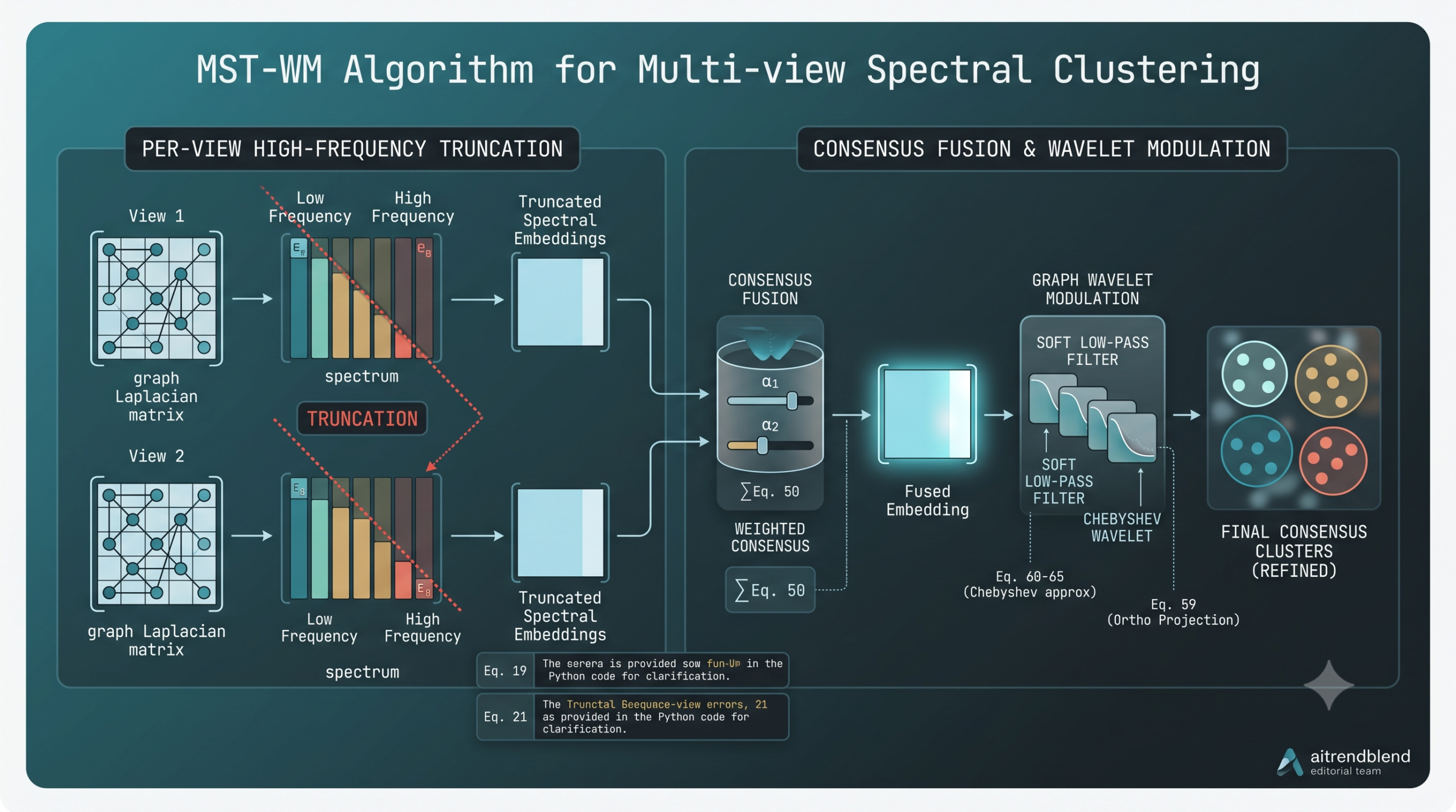
- Built on those two proofs, MST-WM truncates the high frequency component of each view’s graph Laplacian before fusion, then applies a graph wavelet heat-kernel filter to the fused embedding to mop up whatever noise is left.
- Across ten benchmark datasets MST-WM posts the best average accuracy, normalized mutual information, and purity against twelve competing methods, with the largest gains showing up on the noisiest, most heterogeneous datasets rather than the cleanest ones.
Why not every eigenvector deserves the same trust
Clustering data that comes from more than one source, several sensors describing the same object, or several feature extractors run on the same image, is called multi-view clustering, and the whole point is to combine complementary information across those views into one coherent grouping rather than analyzing each view in isolation. Graph based approaches to this problem, generally called multi-view spectral clustering, build a similarity graph for each view and then work with the graph Laplacian, a matrix whose eigenvectors reveal the underlying cluster geometry through spectral decomposition. Methods in this family have grown steadily more sophisticated, from early approaches that impose pairwise consistency constraints across views to methods that automatically learn how much weight each view should get when the graphs get fused together.
The paper’s central observation is that essentially every one of these methods treats a view’s graph Laplacian and its full spectrum as one indivisible object. Once a similarity graph gets built for a view, whatever noise, outliers, or unreliable similarity measurements are baked into that graph get carried forward into every downstream step exactly as faithfully as the genuine signal does. From the perspective of graph signal processing, that is a strange thing to do, because the eigenvectors of a graph Laplacian are not interchangeable. They correspond to different frequency bands, in direct analogy to how a Fourier transform decomposes an ordinary signal into frequency components, and those different bands have been known for some time in the graph signal processing literature to carry qualitatively different kinds of information.
What low and high frequency actually mean on a graph
The eigenvectors associated with small eigenvalues of the graph Laplacian are the low frequency components, and they encode smooth, slowly varying structure across the graph, the kind of broad, global geometry that genuine cluster partitions tend to follow. The eigenvectors associated with large eigenvalues are the high frequency components, and they capture the opposite, sharp local variation, isolated anomalies, and exactly the kind of noise that a messy real world similarity graph tends to be full of. Existing multi-view spectral clustering methods either fuse the entire spectrum wholesale or simply restrict the embedding dimension to match the number of target clusters, without ever explicitly penalizing the high frequency region specifically. The paper argues this is precisely why these methods stay vulnerable to view specific graph disturbances, since nothing in the fusion process stops high frequency noise from one view from bleeding directly into the shared consensus representation.
Proving it rather than just observing it
What sets this paper apart from a purely empirical observation is that it backs the intuition with four formal properties, each with a full proof, rather than treating the low frequency versus high frequency distinction as a heuristic. The setup starts from the standard symmetric normalized graph Laplacian and its eigendecomposition, with eigenvalues ordered from smallest to largest, and the classic spectral clustering objective, minimizing the trace of the embedding matrix transposed times the Laplacian times the embedding matrix, subject to the embedding columns being orthonormal.
Removing low frequency components hurts, provably, in two separate ways
Property 1 shows that if you truncate the Laplacian by removing its lowest frequency eigenvectors and then solve the spectral clustering problem again on what remains, the best achievable objective value can only get worse, never better, because the optimization is forced into a higher energy subspace than the one that actually contained the genuine cluster structure. Property 2 goes a step further and shows the same truncation also makes the resulting embedding measurably more sensitive to any subsequent perturbation, since its local stability now depends on a larger eigenvalue than before, formally confirming that discarding the low frequency subspace does not just lower quality, it also makes the model shakier under any additional noise. Together these two results are a precise mathematical statement of something practitioners have probably suspected informally for a while, that you cannot throw away the low end of the spectrum without real cost.
Removing high frequency components is different, and that difference is the whole point
Property 3 proves the mirror image result for the opposite end of the spectrum. As long as the number of retained eigenvectors still covers the true low frequency clustering subspace, truncating away the highest frequency eigenvectors leaves the optimal spectral clustering solution completely unchanged, exactly the same objective value, exactly the same embedding. Nothing is lost. Property 4 then shows that this same truncation actually improves robustness, formally, by proving that the increase in the clustering objective caused by any perturbation is provably smaller after high frequency truncation than before it, because the difference between the original and truncated Laplacian is positive semidefinite.
Put together, these four properties describe what the paper names the LGH pattern, short for low frequency gain and high frequency attenuation, formalized as a spectral response function that should be positive across the low frequency band and negative across the high frequency band relative to some baseline response. It is a genuinely asymmetric prescription. Preserve and even amplify the low end of the spectrum, because that is where the actual cluster geometry lives, and actively suppress the high end, because that is where instability concentrates, and there is no theoretical reason to expect symmetric treatment of both ends to be the right design choice.
Confirming the theory empirically before building on it
Before proposing a full method, the authors ran a direct empirical test of exactly this asymmetry, using an existing strong spectral clustering baseline called SCALC on the Caltech101-7 dataset. They progressively removed increasing fractions of the spectrum from each end, from zero up to a quarter of all eigenvectors, and tracked accuracy, normalized mutual information, adjusted Rand index, and purity along the way. The result lines up cleanly with the theory. Even a small amount of low frequency removal caused a sharp collapse in every metric, with normalized mutual information and adjusted Rand index both approaching zero once enough low frequency structure was gone, essentially destroying the cluster signal entirely. Removing a moderate amount of high frequency content instead, up to roughly a fifth of the spectrum, left every metric stable or slightly improved, direct evidence that a meaningful chunk of the high frequency band really was carrying more noise than signal.
Turning the theory into a working method
MST-WM, short for Multi-View Spectral Clustering via High-Frequency Truncation and Graph Wavelet Modulation, is built around three coordinated stages that follow directly from the properties above, per-view truncation, consensus fusion, and post-fusion wavelet refinement.
Truncating each view before it ever gets a chance to pollute the others
For every view, the method builds a symmetric normalized graph Laplacian and truncates it by discarding a fixed fraction of its highest frequency eigenvectors, keeping only the lowest frequency components before any embedding or fusion happens at all.
This ordering matters. Truncating at the view level, before fusion, is exactly what stops one view’s unstable, noisy high frequency structure from ever spreading into the shared consensus representation the way it would if the full, untruncated spectrum from every view got fused first and cleaned up only afterward.
Fusing embeddings with weights that favor the more trustworthy views
Each view’s truncated Laplacian produces its own spectral embedding, and these are combined into one consensus embedding through a weighted sum, where the weights are learned rather than fixed. The optimization derives a genuinely elegant closed-form update for these weights, showing that the optimal weight for a view is inversely related to that view’s own spectral clustering cost, so a view whose truncated Laplacian produces a lower, better objective value automatically earns a larger say in the final consensus.
Cleaning up what fusion could not fully remove
Hard truncation at the view level does not necessarily remove every trace of instability, since fusion itself can reintroduce mismatches between views even after each one has been individually cleaned. The final stage applies a graph wavelet operator to the fused embedding, built from a heat-kernel spectral filter that attenuates larger eigenvalues of the fused Laplacian more strongly than smaller ones, functioning as a continuous, soft low-pass filter layered on top of the earlier hard truncation.
Computing this filter directly would require a full eigendecomposition of the fused Laplacian, which gets expensive as datasets grow, so the method approximates the wavelet operator with a Chebyshev polynomial expansion on a rescaled Laplacian instead, avoiding that eigendecomposition entirely while still capturing the same smoothing behavior. The refined embedding is then obtained by an orthogonal Procrustes style projection, essentially finding the closest orthonormal embedding to the wavelet-smoothed result, computed either exactly through a singular value decomposition or, for larger graphs, through the same Chebyshev approximation used for the filter itself.
How the whole thing gets optimized
The full objective, combining the per-view truncated spectral terms, a fusion consistency penalty, the wavelet refinement term, and a regularizer on the view weights, is optimized by block coordinate descent, alternating closed-form updates for the per-view embeddings, the fused embedding, the view weights, and the wavelet-refined embedding until the objective stabilizes. Every one of these subproblems reduces to a familiar linear algebra operation, an eigenvector computation, a convex quadratic program solvable through the KKT conditions, or an orthogonal Procrustes projection, which is part of why the overall procedure converges reliably in practice rather than needing a more fragile, hand-tuned training loop.
How well it actually performs
The team tested on ten benchmark datasets spanning object recognition, handwritten digits, faces, scenes, and cross-domain office images, comparing against twelve baselines split between deep learning approaches and traditional spectral or matrix factorization methods, including a strong recent spectral baseline called SCALC that the paper treats as its most direct point of comparison.
Average results across ten datasets
| Metric | Best deep baseline | SCALC, strongest spectral baseline | MST-WM |
|---|---|---|---|
| Accuracy, average | PIMVC, 0.6770 | 0.7117 | 0.7429 |
| Normalized mutual information, average | UEAF, 0.5729 | 0.6160 | 0.6535 |
| Purity, average | PIMVC, 0.7161 | 0.7397 | 0.7814 |
MST-WM posts the best average score on all three metrics across all ten datasets, and the comparison against SCALC specifically is the more meaningful one, since SCALC is already a strong, purpose built spectral clustering baseline rather than a weak strawman. Beating it consistently suggests the improvement genuinely comes from the explicit frequency management rather than from some unrelated advantage in graph construction or post-processing that a weaker baseline might have lacked.
Where the gains concentrate
| Dataset | SCALC accuracy | MST-WM accuracy | Gain |
|---|---|---|---|
| VOC | 0.5513 | 0.6268 | +0.0755 |
| Scene15 | 0.4153 | 0.4629 | +0.0476 |
| Mfeat | 0.8564 | 0.9059 | +0.0495 |
| 100Leaves | 0.8624 | 0.8793 | +0.0169 |
| UCI-digits | 0.9132 | 0.9291 | +0.0159 |
| ORL | 0.6500 | 0.6826 | +0.0326 |
The pattern here is informative rather than incidental. The largest single gains show up on VOC and Scene15, datasets the paper describes as having stronger view heterogeneity, more complex underlying manifold structure, and noisier local neighborhood relationships, exactly the conditions under which unstable high frequency components would be easiest to introduce by fusing complete, untruncated spectral information. On comparatively cleaner, large-scale handwritten digit datasets like UCI-digits and Mfeat, the improvement is smaller in absolute terms but still consistently positive, which the paper reads as evidence that the framework is not narrowly specialized for messy data but generalizes reasonably well across the cleanliness spectrum, even if its biggest wins are exactly where you would expect frequency-aware noise suppression to matter most.
What the ablation isolates
| Variant | Average accuracy | Average NMI | Average purity |
|---|---|---|---|
| Without high frequency truncation | 0.6098 | 0.5214 | 0.6487 |
| Without graph wavelet modulation | 0.6536 | 0.5361 | 0.6648 |
| Full model | 0.7429 | 0.6535 | 0.7814 |
Removing high frequency truncation costs more than removing graph wavelet modulation does, roughly 13 points of average accuracy against roughly 9, which is a reasonable confirmation that the harder, per-view truncation step carries more of the overall weight, consistent with Properties 3 and 4 identifying it as the mechanism that preserves the clustering subspace exactly while directly reducing perturbation sensitivity. But removing the wavelet modulation alone still costs a meaningful amount, showing that hard truncation by itself is not sufficient and that the softer, continuous smoothing applied after fusion genuinely catches residual noise the hard cutoff missed, particularly any inconsistency introduced by the fusion step itself. Neither component alone reaches the full model’s performance, which is the paper’s basis for calling the two mechanisms complementary rather than redundant.
How sensitive the method is to its own settings
The truncation ratio, how large a fraction of each view’s high frequency spectrum gets removed, shows a clear and theoretically consistent pattern across the parameter sweep. Performance improves as a moderate portion gets truncated and then declines again once the truncation becomes too aggressive, confirming both halves of the theory at once, that some high frequency removal helps and that removing too much eventually starts cutting into genuine local structure the way Property 1 would predict for any component that actually matters. The authors settle on a truncation ratio around 0.15 based on this sweep, with the fusion weight, wavelet regularization strength, and view weight regularization parameters each showing similarly wide, forgiving stable ranges rather than requiring fragile, precise tuning.
Testing the robustness claim directly, not just assuming it
Rather than relying only on the theoretical properties, the team ran a targeted robustness experiment, injecting orthogonal noise directly into the final embedding space produced by every compared method, at escalating intensities, and re-running k-means clustering on the perturbed result each time. Every method’s performance declined as the injected noise grew stronger, which is expected, but the baseline methods showed clearly steeper drops, while MST-WM’s degradation stayed noticeably shallower and more gradual across the same noise range. That is a direct empirical test of exactly what Properties 2 and 4 predicted mathematically, that a method built around preserving low frequency structure while suppressing high frequency instability should hold up better under added perturbation than one that treats the whole spectrum as a single, undifferentiated object, and the experiment backs that prediction up rather than leaving it as an untested theoretical claim.
Honest limitations
The paper names its central limitation plainly rather than glossing over it, performance depends on the truncation ratio, and while the empirical sweep shows a comparatively stable, forgiving range, the actual optimal value can shift depending on how noisy a specific dataset’s views happen to be. The authors flag a genuinely concerning edge case too, in graphs that are already very sparsely connected, aggressive truncation risks discarding structural boundaries that were actually meaningful rather than noise, since a sparse graph has less redundant high frequency content to safely throw away in the first place. The current method also fixes one truncation ratio for every view rather than learning a view-specific threshold, even though different views plausibly carry very different amounts of genuine high frequency noise, which the authors explicitly flag as a direction for future work, an adaptive, data-driven way to learn the best per-view truncation threshold rather than tuning one shared hyperparameter across all views.
A few additional points are worth naming. The theoretical properties are proven specifically for the standard symmetric normalized Laplacian and a hard, sharp frequency cutoff, and while the wavelet stage introduces a softer, continuous filter, the core truncation guarantees rest on the binary in-or-out framing rather than a fully continuous one. The benchmark datasets, while genuinely varied across ten different domains, are all standard multi-view clustering benchmarks rather than newly collected data reflecting some specific, harder real-world deployment scenario, so how the method performs on genuinely novel view combinations outside this test suite remains untested here.
Takeaway for practitioners
If your multi-view clustering pipeline already builds a graph Laplacian per view, adding a hard high frequency truncation step before fusion is a comparatively simple, well justified change to try first, with a real theoretical guarantee, Property 3, that you will not lose any of the genuine low frequency cluster structure as long as you keep enough eigenvectors to cover your target number of clusters.
Takeaway on the theory
The cleanest idea in this paper is that low frequency and high frequency spectral components are not just informally different in character, they are provably asymmetric in their effect on both accuracy and robustness, which turns a design choice that is usually made by intuition or by trial and error into something you can actually reason about with linear algebra.
Where this could go next
The specific contribution here targets multi-view spectral clustering, but the underlying LGH principle, that low frequency graph structure should be preserved or amplified while high frequency structure should be actively attenuated, is a statement about graph signal processing broadly, not something inherently tied to clustering as a task. Any graph based learning method that relies on a Laplacian eigendecomposition and currently treats the full spectrum as one undifferentiated object, single-view spectral methods, certain graph neural network architectures that use spectral graph convolutions, or graph based semi-supervised learning, could in principle benefit from the same asymmetric frequency treatment this paper proves out for the multi-view clustering case specifically.
The honest limitation around per-view truncation tuning is the natural next problem for anyone extending this work. A fixed, shared truncation ratio is a reasonable starting point that the parameter sweep shows is comparatively forgiving, but it leaves real value on the table in settings where views genuinely differ in how much high frequency noise they carry, and the sparse-graph edge case the authors flag is a genuine caveat rather than a minor footnote, since it identifies a concrete condition under which the whole approach’s core assumption, that high frequency content is mostly disposable noise, can actually break down.
What the four proven properties already establish, regardless of how the method gets extended from here, is that the question of which spectral components to trust in graph based clustering has an actual, provable answer rather than only an intuitive one. That is a genuinely useful contribution on its own, independent of whether MST-WM specifically becomes the standard tool for the job.
Read the full paper for the complete proofs of Properties 1 through 4, all ten dataset results, and the convergence and robustness figures.
A minimal NumPy implementation
Below is a compact, runnable sketch of the core pipeline, per-view high frequency truncation, weighted consensus fusion, and a Chebyshev-approximated graph wavelet heat-kernel filter. It favors clarity over matching the paper’s exact optimization loop, and it includes a smoke test on small synthetic multi-view data.
Conclusion
The genuine contribution of this paper is turning an intuition that has probably occurred to plenty of people working with spectral methods, that noisy graphs should not get treated identically to clean ones, into something with an actual mathematical guarantee attached. Property 1 and Property 2 pin down exactly why you cannot casually discard low frequency structure, it provably worsens the clustering objective and provably increases sensitivity to further perturbation. Property 3 and Property 4 pin down the opposite for high frequency structure just as precisely, showing that as long as you retain enough low frequency eigenvectors to cover your target clusters, truncating the noisy end of the spectrum costs you nothing on the objective while measurably buying you robustness.
That asymmetry, formalized as the LGH pattern, is the real idea underneath MST-WM’s specific architectural choices. The per-view truncation step, the inversely-cost-weighted fusion, and the Chebyshev-approximated wavelet refinement are all reasonable, well justified engineering decisions built on top of that asymmetry, but the asymmetry itself is the transferable insight, not the specific implementation.
The results back the theory up rather than merely gesturing at it. Beating a strong existing spectral baseline like SCALC consistently across ten different datasets, with the largest gains concentrated specifically on the noisiest, most heterogeneous ones, is exactly the pattern you would expect to see if explicit frequency management were doing genuine work rather than adding complexity for a marginal, incidental gain. The orthogonal noise robustness experiment closes the loop by testing the theoretical robustness claims directly rather than leaving them as an assumption.
None of this comes without real caveats, and the paper names its central one directly, that the truncation ratio still needs to be chosen, currently shared across every view rather than tuned per view, and that very sparse graphs pose a genuine edge case where the whole premise, that high frequency content is mostly disposable, can start to break down. Neither caveat undercuts what has actually been established here. The question of which parts of a graph’s spectrum deserve trust in clustering now has a provable answer rather than only an empirical one, and that is a foundation other graph based learning methods well beyond multi-view clustering specifically could reasonably build on.
Frequently asked questions
What is multi-view spectral clustering
It is a clustering approach that builds a similarity graph for each of several different feature representations, or views, of the same underlying data, then uses the eigenvectors of each view’s graph Laplacian, its spectral decomposition, to learn a shared consensus grouping that combines information across all the views rather than relying on any single one.
What do low frequency and high frequency mean for a graph Laplacian
Low frequency components are the eigenvectors associated with the smallest eigenvalues of the graph Laplacian, and they encode smooth, global structure that closely tracks genuine cluster boundaries. High frequency components are the eigenvectors associated with the largest eigenvalues, and they tend to capture sharp local variation, outliers, and noise rather than meaningful cluster structure.
Why does removing low frequency components hurt clustering while removing high frequency components does not
The paper proves that the low frequency eigenvectors specifically define the subspace where the true optimal clustering solution lives, so removing them forces the model into a higher energy, less compatible subspace. High frequency eigenvectors sit outside that subspace entirely, so as long as enough low frequency components are kept to cover the target number of clusters, removing the high frequency ones leaves the optimal solution completely unchanged while still reducing sensitivity to noise.
What is graph wavelet modulation doing in this method
After the truncated, per-view embeddings are fused into one consensus representation, a graph wavelet operator built from a heat-kernel spectral filter is applied to that fused embedding as a soft, continuous smoothing step, catching any residual high frequency mismatch that survived the earlier hard truncation, including inconsistencies that fusion itself can introduce between views.
Does this method beat every baseline on every dataset
The paper reports it achieves the best average accuracy, normalized mutual information, and purity across all ten tested datasets when compared against twelve baseline methods, with the largest performance gains concentrated on the noisiest and most view-heterogeneous datasets rather than the cleanest ones.
What is the main limitation of this approach
Performance depends on choosing a truncation ratio that controls how much of each view’s high frequency spectrum gets removed, and while the paper finds a comparatively stable range for this setting, the same ratio is currently applied uniformly across all views rather than learned per view, and the authors note that very sparsely connected graphs are a genuine edge case where aggressive truncation risks discarding meaningful structure rather than only noise.
Ke, S., Gao, Y., Huang, G., and Ma, X. Multi-view spectral clustering via high-frequency truncation and graph wavelet modulation. Knowledge-Based Systems, volume 349, 2026, article 116477, DOI 10.1016/j.knosys.2026.116477. This analysis is based on the published paper and an independent evaluation of its claims.