
Key points
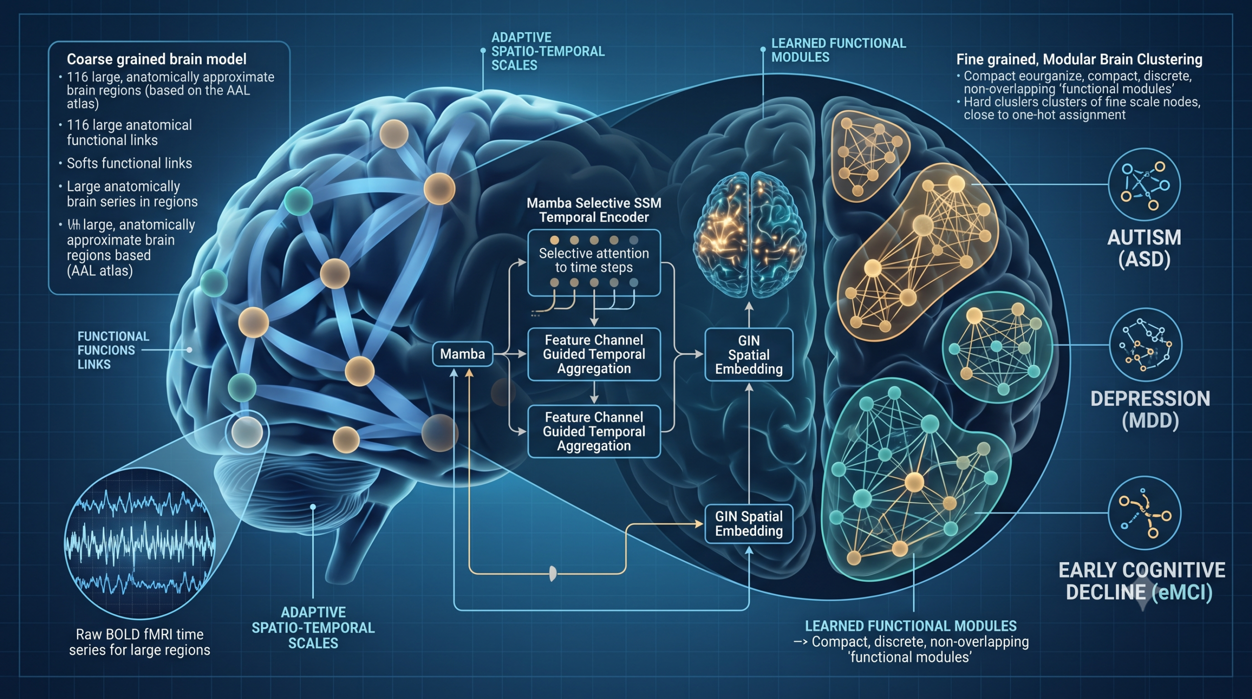
- AdapHBNA processes the same brain scan at several time and space resolutions in sequence, letting a Mamba based temporal encoder guide how the brain is grouped into functional modules rather than fixing that grouping in advance.
- Tested on three real diagnostic tasks, autism spectrum disorder versus typical controls, major depressive disorder versus controls, and early mild cognitive impairment versus controls, the model beat nine comparison methods on accuracy across every dataset reported.
- The gains are real but not universal. On several individual metrics, older and simpler models such as HFBN and STGCN actually scored higher than AdapHBNA, and one comparison against STGCN on the autism dataset did not reach statistical significance.
- The added accuracy comes at a real computational cost. AdapHBNA was the slowest model to train per epoch among everything compared, by a wide margin.
- The authors are candid that their model is not ready for standalone clinical deployment, and lay out concrete next steps including faster inference and testing across many more clinical sites.
The scale problem nobody quite solved
Brain network analysis usually works like this. Take a resting state fMRI scan, split the brain into a fixed number of regions using an anatomical atlas such as AAL with its 116 regions, measure how correlated each region’s activity is with every other region over time, and hand that correlation matrix to a graph neural network or transformer for classification. It is a reasonable pipeline and it has produced a lot of useful research, but it commits to two fixed choices at the very start. The number of regions is whatever the atlas says it is, and the number of time windows, if the model even considers time at all beyond a single static correlation matrix, is whatever a human chose during preprocessing.
The authors argue this is a real mismatch with what the brain actually does. There is a well established idea in neuroscience that brain networks are organized hierarchically, with fine grained regions nesting into broader functional modules, and with neural activity itself unfolding across multiple overlapping timescales rather than one fixed window. A method that locks in a single spatial scale and a single temporal scale before it even starts learning is, in a real sense, fighting the structure of the thing it is trying to model.
Prior attempts at fixing part of this problem exist. Some methods add dynamics by sliding a window across the BOLD time series, but they still use one fixed window size throughout. Others build spatial hierarchies by softly merging fine grained regions into coarser ones, a method called HFBN being the most direct predecessor here, but soft assignment means a single brain region can partially belong to several coarse clusters at once, which makes it hard for a clinician to trace a coarse level finding back to specific anatomy. AdapHBNA tries to fix both problems at the same time, adaptive scale in both time and space, with a hard, unambiguous mapping from fine grained regions up to functional modules.
How the two halves of the model work together
The architecture runs the same two step process inside each of its layers, temporal processing first, spatial processing second, with the output of one becoming the coarser grained input to the next layer. Two real datasets, ABIDE for autism and REST underscore MDD for depression, plus ADNI for early cognitive decline, all get pushed through this pipeline.
Turning a raw BOLD time series into a coarser temporal representation
The first stage encodes the raw signal with Mamba, a selective state space model originally built for efficient long sequence modeling in language tasks. This is, per the authors, the first time Mamba has been applied to encode the temporal dynamics of BOLD signals directly. Unlike a transformer, whose self attention cost grows quadratically with sequence length, Mamba scans through a sequence with linear complexity while still keeping a recurrent memory of everything it has seen, which the authors argue makes it well suited to catching long range dependencies between temporally distant brain states, filtering out short lived noise through its gating mechanism, and prioritizing the diagnostically relevant stretches of a scan without the cost of full attention.
After Mamba encodes the signal, a second and more unusual step happens, something the authors call feature channel guided temporal aggregation. Rather than picking a coarser number of time points by literally averaging adjacent time steps, which is the traditional sliding window approach, the model expands the encoded signal into new channels via a 2D convolution, then uses causal self attention with upper triangular projection matrices to inject temporal meaning into those new channels, ensuring that any given coarse time point can only be influenced by earlier fine grained time points, never later ones. A final mean pooling step collapses this into the actual coarse grained temporal representation that the rest of the layer will use. It is, in effect, learning what a coarser slice of time should look like rather than assuming it is just an average of a fixed window.
Turning brain regions into functional modules with hard, not soft, clustering
Once the temporal side of a layer has produced its coarse grained representation, the spatial side takes over. A brain network is constructed for each subject by treating the coarse grained temporal features as node features, and building an adjacency matrix as the average of a standard Pearson correlation network and a second correlation network built from a learnable linear projection of the same features, so the graph itself is partly hand crafted and partly learned. A graph isomorphism network, GIN, then updates each node’s representation by aggregating information from its neighbors in that graph.
The interesting step is what happens next, called Modular Brain Clustering. Cluster centers representing candidate functional modules are initialized using an orthogonal initialization strategy, then refined during training using two loss terms working together, a dissimilarity loss that pushes different cluster centers apart, and an orthogonality loss that pushes cluster center vectors toward independent directions in feature space, approximating the idea that healthy brain modules should be functionally separate from each other rather than redundant. An assignment matrix is then computed using entmax, a sparsity inducing alternative to softmax, to determine how strongly each fine grained region belongs to each candidate module.
The genuinely distinctive move is what the authors do with that assignment matrix next. Instead of leaving it as a soft, overlapping assignment the way HFBN and DiffPool do, AdapHBNA sharpens it during training toward a hard, close to one hot assignment, meaning each fine grained region is ultimately pushed toward belonging to essentially one coarse module rather than several at once. An entropy based confidence loss drives this sharpening gradually rather than all at once, since the authors found that forcing high confidence too early in training caused the clustering to lock in prematurely before the model had learned anything useful.
What actually happens across the three layers
Each layer repeats this temporal then spatial pattern, progressively shrinking both the number of regions and the temporal resolution, and by the final layer the model has produced a highly compressed, hierarchically organized representation of the brain that gets fed into a standard multilayer perceptron for the actual diagnosis. The total training objective sums four terms, the standard cross entropy classification loss, the dissimilarity loss, the orthogonality loss, and the assignment confidence loss, with the confidence loss weighted by a term that grows over the course of training rather than staying fixed, easing the model into hard assignment rather than forcing it from the first epoch.
The datasets behind the numbers
Three public neuroimaging resources anchor the experiments. ABIDE, used for autism spectrum disorder classification, contributes data from three of its largest sites, NYU with 74 autism cases and 98 controls, UCLA with 48 cases and 37 controls, and UM with 47 cases and 73 controls. REST underscore MDD, used for major depressive disorder classification, contributes three sites as well, Site20 with 282 depression cases and 251 controls, Site21 with 86 cases and 70 controls, and Site25 with 89 cases and 63 controls. ADNI, used for early mild cognitive impairment, contributes 165 cases and 154 controls. All three datasets were preprocessed with the DPARSF pipeline, parcellated primarily using the 116 region AAL atlas, with a secondary set of experiments using the 200 region CC200 atlas to test robustness to a different parcellation scheme.
Training used a fifteen percent held out test set, with the remaining eighty five percent run through five fold cross validation, each fold splitting eighty percent for training and twenty percent for validation. The model trained for 40 epochs with a batch size of 21 and a weight decay of 0.0001. Seven metrics were tracked throughout, accuracy, sensitivity, specificity, F1 score, precision, area under the curve, and balanced accuracy.
The comparison results, and where the model does not simply win everything
AdapHBNA was compared against nine methods split into two groups, established brain network methods including BrainGNN, STGCN, BNT, and HFBN, and general purpose graph and sequence models adapted to this task including GIN, GCN, GAT, plain Mamba without the hierarchical machinery, and DiffPool. Here is how the accuracy numbers stacked up on the four sites reported for the primary autism and depression tasks.
| Site | Task | Best comparison method, accuracy | AdapHBNA accuracy |
|---|---|---|---|
| NYU, ABIDE | Autism vs control | STGCN, 72.1 percent | 75.0 percent |
| UM, ABIDE | Autism vs control | BNT, 71.4 percent | 71.8 percent |
| Site21, REST_MDD | Depression vs control | BNT, 60.1 percent | 65.9 percent |
| Site25, REST_MDD | Depression vs control | HFBN, 60.0 percent | 62.6 percent |
| ADNI | Early cognitive impairment vs control | HFBN and BrainGNN, tied around 72.1 percent | 79.6 percent |
That table tells a genuinely positive story for AdapHBNA on the headline metric, and the margin on ADNI in particular, roughly seven and a half percentage points over the next best method, is a substantial gap rather than a marginal one. But a closer look at the full seven metric tables reveals a more textured picture than accuracy alone suggests, and it is worth walking through because it is exactly the kind of nuance a reader would not get from the abstract.
Where older models actually beat AdapHBNA on individual metrics
On the NYU autism site, HFBN reached a specificity of 94.2 percent, dramatically higher than AdapHBNA’s 77.5 percent, meaning HFBN was considerably better at correctly ruling out autism in controls, even though its overall accuracy of 65.7 percent trailed AdapHBNA by nearly ten points because its sensitivity for actually detecting autism cases was comparatively weak. On the UM autism site, STGCN posted a specificity of 85.0 percent against AdapHBNA’s 69.2 percent, again a real tradeoff, since STGCN’s overall accuracy of 65.0 percent was still well behind AdapHBNA’s 71.8 percent because of weaker sensitivity.
The depression sites tell a similar story. On Site21, HFBN reached a sensitivity of 87.7 percent, far above AdapHBNA’s 66.6 percent, but HFBN’s overall accuracy of 53.3 percent was barely above chance because its specificity collapsed to 51.9 percent, meaning it was flagging a lot of controls as depressed along with the real cases. On Site25, HFBN’s precision of 68.8 percent actually beat AdapHBNA’s 63.9 percent. And on the ADNI task, HFBN’s sensitivity of 82.4 percent outpaced AdapHBNA’s 79.1 percent, though again its much weaker specificity, 60.9 percent against AdapHBNA’s 67.8 percent, dragged its overall balanced performance down.
None of this undercuts the case for AdapHBNA as the strongest all around performer here, since accuracy, F1, and AUC, the metrics that best summarize overall diagnostic quality, consistently favor it. But a reader deciding whether to build on this work should know that no single method in this comparison dominates every metric, and that older, simpler models sometimes trade a large amount of specificity for sensitivity or vice versa in ways that particular clinical use cases might actually prefer over a more balanced but less extreme model.
Statistical significance, and the one comparison that did not clear the bar
The authors ran pairwise significance tests between AdapHBNA and six of the comparison methods on both the ABIDE and REST underscore MDD datasets. On REST underscore MDD, every comparison reached statistical significance at the 0.05 level, with several comparisons reaching p values below 0.001. On ABIDE, five of six comparisons were significant, but the comparison against STGCN specifically did not clear the bar, landing at a p value of 0.08. That is a small but real caveat on an otherwise strong autism result, and it lines up with the accuracy table itself, where STGCN was the closest competitor on the NYU site specifically.
What the ablation and sensitivity experiments add
The authors tested five stripped down variants of their own model, removing the Mamba temporal encoder, removing the coarser scaled temporal aggregation step, removing both temporal components together, removing the graph based spatial embedding, and swapping the order of temporal and spatial processing. The full model consistently outperformed every variant, and the version missing both temporal components performed worst of all, which the authors read as evidence that raw BOLD signals are simply too noisy and unevenly distributed in time to feed directly into spatial clustering without some temporal structuring first.
Two tunable ratios control how aggressively the model compresses information at each layer, a temporal aggregation ratio and a spatial aggregation ratio, both searched over a range and both landing at an optimal value of 0.6 in the reported experiments. At that spatial setting, after two clustering layers roughly thirty six percent of the original 116 regions worth of information is retained in the coarsest representation, which the authors note lines up reasonably well with earlier findings elsewhere in the literature that brain network sparsification tends to work best when around thirty percent of connections are pruned.
Depth also mattered in a way that argues against simply stacking more layers. Going from one layer to two improved accuracy, AUC, and F1 across every dataset tested, but adding a third layer made performance worse everywhere while substantially increasing parameter count and memory use, a fairly clean case of diminishing and then negative returns as the model gets deeper.
Testing whether the model generalizes at all
A few extra experiments push on generalization specifically. Swapping the AAL atlas for the CC200 atlas, which carves the brain into roughly 200 regions instead of 116, produced broadly comparable though slightly lower accuracy on most sites, for instance 72.9 percent on NYU and 69.1 percent on UM under CC200 against 75.0 percent and 71.8 percent respectively under AAL, suggesting the framework is not overly dependent on one specific parcellation scheme but does lose a little ground when the anatomical starting point changes.
A separate cross site test is more directly relevant to real world deployment. The authors took the data driven, coarse grained brain atlas that AdapHBNA learns from its assignment matrices on one set of sites, then applied that learned atlas to a genuinely unseen site the model had never trained on, UCLA for autism and Site20 for depression. A plain GIN model using this externally learned atlas, labeled GIN A in the paper, modestly outperformed the same GIN model using raw, unaggregated features, for example 63.1 percent accuracy against 60.0 percent on the unseen UCLA site. That is a real if modest signal that the functional modules AdapHBNA discovers carry some information that transfers across sites rather than being purely an artifact of the training data, though it is a considerably smaller test than a full multi site validation would be.
What the discriminative regions look like
By sparsifying the learned brain networks down to their most discriminative connections and visualizing them, the authors report that connections among the superior, middle, and inferior frontal gyrus, regions tied to executive function and language, showed up prominently for the autism classification task, consistent with prior autism neuroimaging literature they cite. For depression, regions including the anterior cingulate gyrus, amygdala, hippocampus, and inferior temporal gyrus stood out, again broadly consistent with existing depression research, alongside a finding involving the supplementary motor area that the authors flag as a less expected result worth further study.
Clinical translation gap
The authors themselves are unusually direct about how far this is from a deployable clinical tool, dedicating a specific section of their discussion to what they call clinical translatability. They state plainly that AdapHBNA shows promise for inference speed and memory efficiency on standard hardware, and that it produces interpretable outputs that could support standard rs fMRI workflows, but that fully standalone real time clinical deployment remains genuinely difficult, largely because integrating and validating additional non imaging clinical data alongside the brain scan within one unified system has not been solved here. They name concrete next steps rather than vague promises, targeting inference latency under 500 milliseconds through model compression, and pursuing large scale validation across many more clinical sites before the framework could reasonably be considered a near real time auxiliary tool for clinicians, explicitly framed as auxiliary rather than autonomous.
That framing matters. Every dataset used here, ABIDE, REST underscore MDD, and ADNI, is a public research collection assembled specifically to support method development, not a representative sample of every patient population, healthcare setting, or scanner type a deployed system would eventually encounter. The model was also trained and evaluated with identical hyperparameters copied directly from the autism and depression experiments onto the memory impairment task, with no dataset specific tuning, which the authors present as evidence of generalizability, and it is a reasonable point in that direction, but it also means no one has yet tried to squeeze out the best possible performance specifically for early cognitive decline detection, which a real clinical deployment would likely require.
Clinical limitations
A few limitations deserve to be named plainly rather than left implicit. Site to site sample sizes vary considerably, from just 37 controls at UCLA to 282 depression cases at Site20, and standard deviations on several metrics, particularly on the smaller depression sites, run into the double digits, meaning results likely varied a great deal across the five cross validation folds and would benefit from a larger and more evenly distributed sample before anyone treats these accuracy numbers as stable. The computational cost is also a genuine practical barrier right now. Table 8 in the paper shows AdapHBNA took 6.234 seconds per training epoch on an NVIDIA RTX 4090, meaningfully slower than every other method compared, including STGCN at 0.385 seconds and even plain Mamba at 2.82 seconds, a real hardware and turnaround time cost that the authors’ own stated goal of sub 500 millisecond inference has not yet addressed, since that goal is about inference speed rather than training speed and remains future work.
It is also worth being honest that grouping the entire NYU, UCLA, and UM datasets under one ASD label, or the entire REST underscore MDD sites under one MDD label, treats these conditions as single, uniform categories, when autism spectrum disorder in particular spans an enormous range of presentations and support needs, and major depressive disorder varies significantly in severity and subtype. A model that distinguishes an average autistic brain scan pattern from an average non autistic one is not the same thing as a tool that could meaningfully characterize where any individual person sits on that spectrum, and the paper does not claim otherwise, but it is an important distinction for any reader thinking about what a result like this can and cannot tell us about an actual person.
Where this leaves brain network research
The most transferable idea in this paper is not really about brains specifically. It is the argument that letting temporal structure guide spatial structure, rather than treating them as two independent design choices bolted together, produces a better representation than picking one fixed scale for each and hoping for the best. That argument is backed up by a genuinely careful ablation study, and the consistent accuracy improvement across three quite different diagnostic tasks, autism, depression, and early cognitive decline, using the exact same hyperparameters each time, is a meaningfully stronger generalization claim than most single dataset papers can make.
The honest complication is that this improvement is not free and not uniform. It costs meaningfully more compute per epoch than every comparison method, it does not beat every baseline on every individual metric, one comparison against a strong recent baseline did not reach statistical significance on one of the two primary datasets, and the model has, in the authors’ own words, real work remaining before it could function as even an auxiliary clinical tool. None of that is a knock against the paper. If anything, a paper that names its own computational cost, reports the metrics where a simpler competitor wins, and states outright that standalone clinical deployment is not yet feasible is doing exactly the kind of careful reporting that this field could use more of.
A PyTorch implementation of the architecture
The code below reconstructs the core mechanisms of AdapHBNA as described in the paper and its appendix, a simplified Mamba style selective state space encoder following the paper’s own equations, the feature channel guided coarser temporal aggregation step with causal self attention, GIN based spatial embedding, and Modular Brain Clustering with its dissimilarity, orthogonality, and assignment confidence losses. The selective scan is implemented as an explicit loop over time steps for clarity rather than a fused hardware level kernel, and the entmax sparsity function is approximated with a simple thresholded softmax, both noted in comments, since the goal here is a readable, runnable reconstruction rather than a production grade reimplementation of the original codebase.
# adaphbna.py
# Reconstruction of AdapHBNA from Wang et al., Neural Networks 205 (2027) 109305
# This is an independent, simplified reimplementation for educational purposes,
# not the authors' original code. The selective scan and entmax steps are
# simplified for readability, noted inline where they diverge from the paper.
import torch
import torch.nn as nn
import torch.nn.functional as F
import math


class SelectiveSSM(nn.Module):
    """A simplified selective state space scan following the paper's Appendix A.1 equations,
    A_bar = exp(delta A), B_bar approximated with the zero order hold formula,
    looped explicitly over time for clarity rather than a fused kernel."""
    def __init__(self, channels, state_size=16):
        super().__init__()
        self.state_size = state_size
        self.A_log = nn.Parameter(torch.randn(channels, state_size) * 0.1 - 1.0)
        self.linear_b = nn.Linear(channels, state_size)
        self.linear_c = nn.Linear(channels, state_size)
        self.linear_delta = nn.Linear(channels, channels)

    def forward(self, x):
        # x shape, batch by channels by time
        batch, channels, T = x.shape
        A = -torch.exp(self.A_log)
        x_t = x.transpose(1, 2)
        delta = F.softplus(self.linear_delta(x_t))
        B = self.linear_b(x_t)
        C = self.linear_c(x_t)

        h = torch.zeros(batch, channels, self.state_size, device=x.device)
        outputs = []
        for t in range(T):
            delta_t = delta[:, t, :].unsqueeze(-1)
            a_bar = torch.exp(delta_t * A.unsqueeze(0))
            b_bar = delta_t * B[:, t, :].unsqueeze(1)
            h = a_bar * h + b_bar * x_t[:, t, :].unsqueeze(-1)
            y_t = (h * C[:, t, :].unsqueeze(1)).sum(dim=-1)
            outputs.append(y_t)
        y = torch.stack(outputs, dim=2)
        return y


class MambaBlock(nn.Module):
    """Follows Eq. A.3 to A.5, split projection, conv1d and silu on the main branch,
    silu gating branch, selective SSM, then a merge projection back to channel dim."""
    def __init__(self, channels):
        super().__init__()
        self.in_proj = nn.Linear(channels, channels * 2)
        self.conv1d = nn.Conv1d(channels, channels, kernel_size=3, padding=1, groups=channels)
        self.ssm = SelectiveSSM(channels)
        self.out_proj = nn.Linear(channels, channels)
        self.norm = nn.LayerNorm(channels)

    def forward(self, x):
        # x shape, batch by channels by time
        x_t = x.transpose(1, 2)
        projected = self.in_proj(x_t)
        u, res = projected.chunk(2, dim=-1)
        u = F.silu(self.conv1d(u.transpose(1, 2)))
        res = F.silu(res.transpose(1, 2))
        ssm_out = self.ssm(u)
        merged = ssm_out * res
        out = self.out_proj(merged.transpose(1, 2))
        # A residual connection plus layer norm keeps activations stable across
        # stacked hierarchy layers during this smoke test
        out = self.norm(out + x_t)
        return out.transpose(1, 2)


class TemporalHierarchicalAggregation(nn.Module):
    """Channel expansion followed by causal self attention with upper triangular
    projections, then mean pooling to a coarser temporal scale, following Eq. 2 to 5."""
    def __init__(self, n_rois, t_fine, t_coarse):
        super().__init__()
        self.t_coarse = t_coarse
        self.channel_expand = nn.Conv2d(1, t_coarse, kernel_size=1)
        # W3 and W3 prime map from the fine temporal dimension to the coarse one,
        # matching the paper's rectangular upper triangular ULinear Projection matrices
        self.w3 = nn.Parameter(torch.randn(t_fine, t_coarse) * 0.05)
        self.w3_prime = nn.Parameter(torch.randn(t_fine, t_coarse) * 0.05)

    def forward(self, m):
        # m shape, batch by n_rois by t_fine, the Mamba encoded representation
        batch, n_rois, t_fine = m.shape
        m_prime = self.channel_expand(m.unsqueeze(1))
        # m_prime shape, batch by t_coarse by n_rois by t_fine
        w3_causal = torch.triu(self.w3)
        w3p_causal = torch.triu(self.w3_prime)
        # Summarize each surrogate coarse channel to build the causal temporal attention
        summary = m_prime.mean(dim=2)
        # summary shape, batch by t_coarse by t_fine
        q = torch.matmul(summary, w3_causal)
        k = torch.matmul(summary, w3p_causal)
        # q and k shape, batch by t_coarse by t_coarse after the projection
        scores = torch.matmul(q, k.transpose(-1, -2)) / math.sqrt(self.t_coarse)
        a_t = F.softmax(scores, dim=-1)
        # a_t shape, batch by t_coarse by t_coarse, mixes the surrogate coarse channels
        m_double_prime = torch.einsum("bij,bjrf->birf", a_t, m_prime)
        m_hat = m_double_prime.mean(dim=3)
        # m_hat shape, batch by t_coarse by n_rois, the coarse grained temporal representation
        return m_hat


class GINSpatialEmbedding(nn.Module):
    """Follows Eq. 6, H = MLP([(1+eps) I + A_g] M_hat^T), with A_g built as the
    average of a Pearson correlation network and a learnable projected correlation network."""
    def __init__(self, t_coarse, hidden_dim):
        super().__init__()
        self.eps = nn.Parameter(torch.zeros(1))
        self.task_proj = nn.Linear(t_coarse, t_coarse)
        self.mlp = nn.Sequential(
            nn.Linear(t_coarse, hidden_dim),
            nn.ReLU(inplace=True),
            nn.Linear(hidden_dim, hidden_dim),
        )
        self.norm = nn.LayerNorm(hidden_dim)

    def _correlation(self, x):
        x_centered = x - x.mean(dim=2, keepdim=True)
        cov = torch.bmm(x_centered, x_centered.transpose(1, 2))
        std = x_centered.std(dim=2, keepdim=True) + 1e-6
        corr = cov / (std @ std.transpose(1, 2))
        return corr

    def forward(self, m_hat):
        # m_hat shape, batch by t_coarse by n_rois
        m_hat_t = m_hat.transpose(1, 2)
        # m_hat_t shape, batch by n_rois by t_coarse, node features
        pc_network = self._correlation(m_hat_t)
        task_adaptive = self._correlation(self.task_proj(m_hat_t))
        a_g = 0.5 * pc_network + 0.5 * task_adaptive
        n_rois = a_g.shape[1]
        identity = torch.eye(n_rois, device=m_hat.device).unsqueeze(0)
        aggregated = (1 + self.eps) * identity + a_g
        h = self.norm(self.mlp(torch.bmm(aggregated, m_hat_t)))
        return h, a_g


def approximate_entmax(logits, dim=-1):
    # Simplified stand in for entmax, a sparsity inducing softmax variant.
    # Real entmax solves a threshold projection, here we approximate the
    # sparsifying effect with a squared relu normalization for readability.
    relu_sq = F.relu(logits) ** 2
    return relu_sq / (relu_sq.sum(dim=dim, keepdim=True) + 1e-8)


class ModularBrainClustering(nn.Module):
    """Cluster centers refined with dissimilarity and orthogonality losses,
    Eq. A.6 and A.7, plus a hard assignment confidence loss, Eq. 8 and 9."""
    def __init__(self, n_rois, hidden_dim, n_clusters):
        super().__init__()
        self.n_clusters = n_clusters
        self.centers = nn.Parameter(torch.randn(n_clusters, hidden_dim) * 0.1)
        self.w_d = nn.Linear(hidden_dim, hidden_dim)
        self.w_e = nn.Linear(hidden_dim, hidden_dim)

    def forward(self, h):
        # h shape, batch by n_rois by hidden_dim, node embeddings from GIN
        projected = F.relu(self.w_e(F.relu(self.w_d(h))))
        centers_norm = self.centers / (self.centers.norm(dim=1, keepdim=True) + 1e-8)
        logits = torch.einsum("brd,cd->brc", projected, centers_norm)
        s = approximate_entmax(logits, dim=-1)
        x_coarse = torch.einsum("brc,brd->bcd", s, h)
        return x_coarse, s

    def dissimilarity_loss(self):
        diffs = self.centers.unsqueeze(0) - self.centers.unsqueeze(1)
        sq_dists = (diffs ** 2).sum(-1)
        mask = 1 - torch.eye(self.n_clusters, device=self.centers.device)
        return -(sq_dists * mask).sum() / (self.n_clusters * (self.n_clusters - 1) + 1e-8)

    def orthogonality_loss(self):
        centers_norm = self.centers / (self.centers.norm(dim=1, keepdim=True) + 1e-8)
        sim = centers_norm @ centers_norm.t()
        mask = 1 - torch.eye(self.n_clusters, device=self.centers.device)
        return ((sim ** 2) * mask).sum() / (self.n_clusters * (self.n_clusters - 1) + 1e-8)

    def confidence_loss(self, s, temperature=0.5):
        s_sq = s ** 2
        s_target = s_sq / (s_sq.sum(dim=1, keepdim=True) + 1e-8)
        s_target = approximate_entmax(s_target / temperature, dim=-1)
        align = (s_target * torch.log((s_target + 1e-8) / (s + 1e-8))).sum(dim=(1, 2)).mean()
        q = s.sum(dim=1)
        q = q / (q.sum(dim=-1, keepdim=True) + 1e-8)
        entropy = -(q * torch.log(q + 1e-8)).sum(dim=-1).mean()
        return align + entropy


class AdapHBNALayer(nn.Module):
    def __init__(self, n_rois_in, n_rois_out, t_in, t_out, hidden_dim):
        super().__init__()
        self.mamba = MambaBlock(n_rois_in)
        self.temporal_agg = TemporalHierarchicalAggregation(n_rois_in, t_in, t_out)
        self.spatial_embed = GINSpatialEmbedding(t_out, hidden_dim)
        self.clustering = ModularBrainClustering(n_rois_in, hidden_dim, n_rois_out)

    def forward(self, x):
        # x shape, batch by n_rois_in by t_in
        m = self.mamba(x)
        m_hat = self.temporal_agg(m)
        h, a_g = self.spatial_embed(m_hat)
        x_coarse, s = self.clustering(h)
        losses = {
            "dissimilarity": self.clustering.dissimilarity_loss(),
            "orthogonality": self.clustering.orthogonality_loss(),
            "confidence": self.clustering.confidence_loss(s),
        }
        return x_coarse, losses


class AdapHBNA(nn.Module):
    def __init__(self, n_rois=116, t_series=200, hidden_dim=32, n_classes=2, spatial_ratio=0.6, temporal_ratio=0.6, n_layers=2):
        super().__init__()
        layers = []
        n_current, t_current = n_rois, t_series
        for layer_idx in range(n_layers):
            n_next = max(int(n_current * spatial_ratio), 2)
            t_coarse = max(int(t_current * temporal_ratio), 2)
            layers.append(AdapHBNALayer(n_current, n_next, t_current, t_coarse, hidden_dim))
            n_current = n_next
            # After layer 0, GIN turns each node into a hidden_dim length feature vector,
            # so the next layer's Mamba encoder treats hidden_dim as its time dimension
            t_current = hidden_dim
        self.layers = nn.ModuleList(layers)
        self.classifier = nn.Sequential(
            nn.Linear(hidden_dim, hidden_dim),
            nn.ReLU(inplace=True),
            nn.Linear(hidden_dim, n_classes),
        )

    def forward(self, x):
        # x shape, batch by n_rois by t_series, raw BOLD signals
        all_losses = []
        current = x
        for layer in self.layers:
            current, losses = layer(current)
            all_losses.append(losses)
        pooled = current.mean(dim=1)
        logits = self.classifier(pooled)
        return logits, all_losses


def total_loss(logits, labels, all_losses, lam=0.001, epoch=0):
    ce = F.cross_entropy(logits, labels)
    beta = 1 - math.exp(-2 * epoch)
    ld = sum(l["dissimilarity"] for l in all_losses)
    lo = sum(l["orthogonality"] for l in all_losses)
    lh = sum(l["confidence"] for l in all_losses)
    return ce + lam * ld + lam * lo + beta * lh


def evaluate(model, x, y):
    model.eval()
    with torch.no_grad():
        logits, _ = model(x)
        preds = logits.argmax(dim=-1)
        acc = (preds == y).float().mean().item()
    model.train()
    return acc


if __name__ == "__main__":
    # Smoke test on dummy data shaped like the paper's AAL parcellation,
    # 116 ROIs, a shortened time series for a fast test, two class diagnosis.
    torch.manual_seed(0)
    batch_size, n_rois, t_series, n_classes = 4, 116, 64, 2
    dummy_x = torch.randn(batch_size, n_rois, t_series)
    dummy_y = torch.randint(0, n_classes, (batch_size,))

    model = AdapHBNA(n_rois=n_rois, t_series=t_series, hidden_dim=16, n_classes=n_classes)
    optimizer = torch.optim.Adam(model.parameters(), lr=0.0006, weight_decay=0.0001)

    for epoch in range(3):
        logits, all_losses = model(dummy_x)
        loss = total_loss(logits, dummy_y, all_losses, epoch=epoch)
        optimizer.zero_grad()
        loss.backward()
        optimizer.step()
        acc = evaluate(model, dummy_x, dummy_y)
        print(f"epoch {epoch} loss {loss.item():.4f} dummy accuracy {acc:.4f}")

    print("Smoke test complete, shapes and gradients flow end to end through both hierarchy levels.")
Conclusion
The core achievement of this paper is a genuinely unified answer to a design question that most brain network analysis methods have quietly punted on, how coarse should the model’s view of space and time be, and should that choice be fixed in advance or learned from the data. AdapHBNA answers by learning both, letting a Mamba based temporal encoder shape the input that a modular clustering step then organizes into hard, anatomically traceable functional modules, and repeating that process across layers so the model builds up a genuinely hierarchical picture rather than committing to one resolution from the start. Testing that same architecture, with the same hyperparameters, across three quite different diagnostic tasks and coming out ahead on accuracy every time is a stronger piece of evidence for the idea than a single dataset result would have been.
The conceptual shift worth carrying into other work is treating the choice of spatial and temporal scale as something a model learns rather than something a researcher sets once during preprocessing and never revisits. That idea is not tied to brain imaging specifically. Any domain where a signal has both a natural but uncertain granularity in space, sensor networks, climate grids, financial market structures, and a natural but uncertain granularity in time could plausibly benefit from a temporal encoder that hands off a data driven coarse resolution to a spatial clustering step, rather than a human choosing both numbers ahead of time.
What the paper does not settle, and says so plainly in its own discussion, is what happens when this framework has to work outside the tidy conditions of a public research dataset, alongside other clinical information, on hardware that has to respond in real time, and across enough sites and scanner types to be confident the discovered functional modules are not simply an artifact of how these three specific datasets happened to be collected. The authors name concrete next steps rather than leaving that as an open question, targeting faster inference through model compression and larger multi center validation, which is a reasonable and specific research agenda rather than a vague promise.
The honest remaining limitation, again one the paper states rather than hides, is that a computational method this much slower to train than every comparison model, this dependent on public datasets with real sample size imbalances across sites, and this early in its path toward handling real clinical data alongside imaging, is a meaningful distance from something a hospital could use tomorrow. That does not diminish what has been shown here. It is a careful, well ablated piece of architecture research with a genuinely novel idea at its center, and the honesty about its own current limits is, if anything, a point in its favor rather than against it.
For a field that has spent a long time treating spatial and temporal modeling of brain networks as two separate problems to be solved independently and then bolted together, a framework that couples them from the start, with hard interpretable clustering instead of soft ambiguous assignment, is a meaningful step, and the fact that the authors made their code public means the open questions they identify are ones the next paper can actually go test.
Honest limitations
Beyond the clinical limitations covered above, a few methodological points deserve mention. All experiments used identical hyperparameters, a learning rate of 0.0006, two layers, a temporal aggregation ratio and spatial aggregation ratio both at 0.6, copied across all three diagnostic tasks with no dataset specific tuning, which supports the generalizability argument the authors make but also means none of the individual results necessarily reflect the best possible performance achievable on any one task specifically. The comparison methods were also not individually retuned with an equally exhaustive hyperparameter search, a reasonable choice for a fair head to head test but one that leaves open whether the gap to, say, STGCN or BNT would shrink under more aggressive tuning of those baselines specifically. Finally, the significance testing reported covers six of the nine comparison methods on each dataset, and does not report significance testing against GIN, GCN, or GAT specifically, so the strength of AdapHBNA’s advantage over those particular baselines rests on the accuracy tables alone rather than a formal statistical test.
Frequently asked questions
What does AdapHBNA stand for and what problem does it solve
Adaptive Hierarchical spatio temporal Brain Network Analysis. It addresses the fact that most brain network models pick one fixed number of brain regions and one fixed time window before training even starts, when real brain activity is organized across many overlapping scales of both space and time.
Which conditions was the model tested on
Three tasks using three public datasets, autism spectrum disorder versus typical controls on the ABIDE dataset, major depressive disorder versus controls on the REST underscore MDD dataset, and early mild cognitive impairment versus controls on the ADNI dataset.
Did AdapHBNA beat every other method on every measurement
No. It led on accuracy, F1 score, and area under the curve across the datasets reported, but several older models beat it on specific individual metrics such as specificity or sensitivity on particular sites, and one comparison against STGCN on the autism dataset did not reach statistical significance.
What is Modular Brain Clustering and why does it use hard assignment
It is the part of the model that groups fine grained brain regions into coarser functional modules. Unlike earlier methods that let a region partially belong to several modules at once, AdapHBNA pushes each region toward belonging to essentially one module, which the authors argue makes it easier to trace a coarse level finding back to specific anatomy.
Is this ready to be used to diagnose autism, depression, or memory problems in a clinic
No. The authors themselves state that standalone real time clinical deployment remains difficult, and they list concrete future work including faster inference and testing across many more clinical sites before anything like that would be appropriate. This is research grade work evaluated on public research datasets, not a clinical diagnostic tool.
Where can I read the original paper and get the code
The paper is published in Neural Networks, volume 205, 2027, article 109305, and the authors’ code is available on their linked GitHub repository referenced in the paper itself.
Read the full paper for the complete mathematical appendix, the additional site level tables, and the discriminative connectivity visualizations.
Read the paper View the codeReaders who want the full mathematical detail rather than this summary can find it at the DOI link for Wang and colleagues in Neural Networks, including the complete appendix equations and the per site significance tables referenced above.
This analysis is based on the published paper and an independent evaluation of its claims.