
Key points
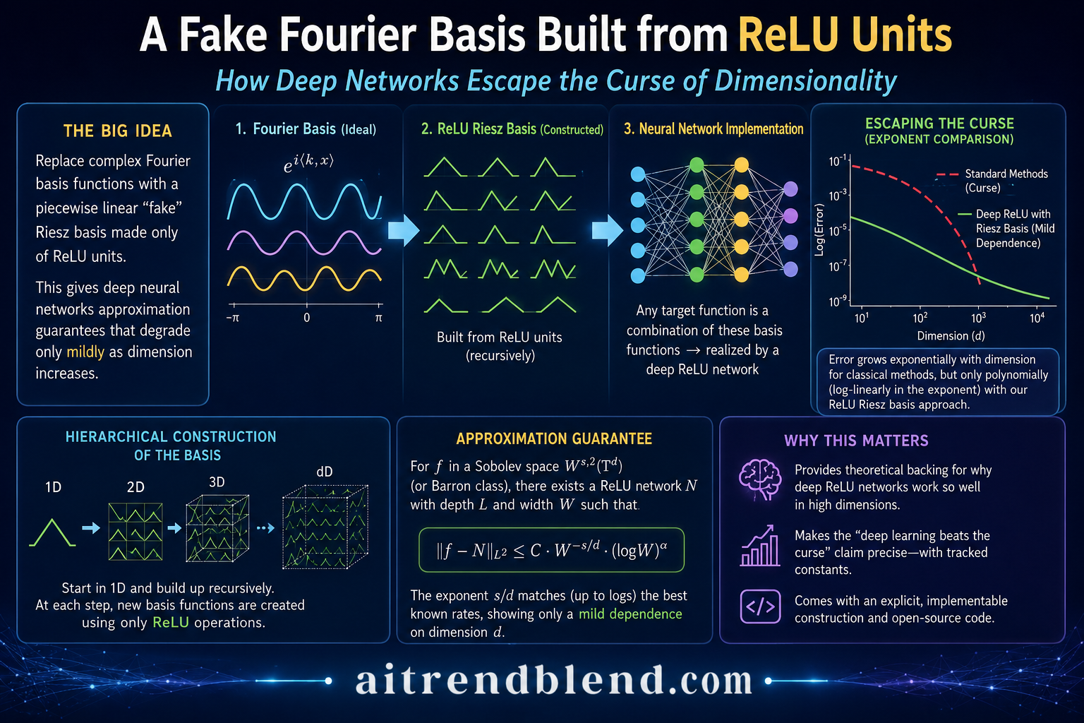
- The paper builds on a 2022 discovery that a pair of piecewise linear functions, shaped like a triangle wave and a trapezoid wave, form a Riesz basis of square integrable functions on the unit interval, much like sine and cosine do, and that these functions can be reproduced exactly by small ReLU networks.
- The authors prove this same system remains a valid basis for Sobolev spaces and Barron classes, the two function spaces most often used to measure how smooth a target function is when studying neural network approximation.
- Because the basis is nonlocal, meaning each basis function is defined across the whole domain rather than only on a small patch, the resulting approximation bounds keep their constants under control as the input dimension grows, unlike wavelet based or Taylor based proofs.
- The paper reproves known approximation rates for both function classes and, in one clean regime, shows the number of network parameters needed grows only polynomially in the dimension rather than exponentially.
- A companion result shows how to approximate these functions using only scattered sample values, connecting the theory to a more realistic setting where a network is trained on data rather than handed a full description of the target function.
- A key supporting lemma solves a variant of the two century old Gauss circle problem, counting lattice points inside a high dimensional ball, in a form that holds for every dimension rather than only in the limit.
The quiet scandal in neural network approximation theory
Ask any expressivity theorist why deep networks are believed to handle high dimensional problems well, and Barron’s 1993 paper comes up almost immediately. Andrew Barron showed that a shallow network with N neurons can approximate a certain class of functions, now called Barron classes, to within error proportional to one over the square root of N, and crucially that rate does not degrade as the input dimension grows. That result is genuinely remarkable, since ordinary linear approximation methods such as polynomials or splines get exponentially worse as dimension increases, a phenomenon known as the curse of dimensionality.
The trouble is that Barron’s result, and most of what followed it for functions with more general smoothness such as Sobolev spaces, was traditionally proven using local approximation techniques. Think of chopping the domain into small patches, approximating the function separately on each patch using a partition of unity or a Taylor expansion, then stitching the pieces together. That approach works, but the stitching step tends to introduce constants that blow up exponentially with dimension, precisely because the number of patches needed to cover a d dimensional cube at a fixed resolution grows exponentially in d. Authors often acknowledge this and move on, since making the dependence explicit is a lot of extra bookkeeping for a result that is already hard to prove.
An unlikely stand in for the Fourier basis
The starting point for this paper is a 2022 result from Daubechies, DeVore, Foucart, Hanin and Petrova. They defined two periodic, piecewise linear functions on the unit interval, one that interpolates a cosine wave at the points zero, one quarter, one half, three quarters and one, and another that interpolates a sine wave at the same points. Call them C and S. Scale them by an integer frequency k to get functions Ck and Sk, and it turns out the whole collection behaves almost exactly like the classical trigonometric basis, satisfying a Riesz basis inequality.
The Riesz basis inequality, saying the energy of any combination of these triangle wave functions is sandwiched between two fixed multiples of the energy of its coefficients, exactly the property that makes Fourier series so useful.
What makes this more than a curiosity is that C and S are literally piecewise linear with a small number of pieces, and every piecewise linear function of one variable can be written exactly as a composition and sum of ReLU units. Daubechies and colleagues showed precisely how, giving a construction where reproducing Ck takes a number of layers that grows only logarithmically in k, using just two neurons per layer. Schneider and Vybíral then extended the whole idea to functions of several variables in 2024, defining a multivariate version built from dot products k times x, and showing the same Riesz basis property holds in every dimension with constants that do not degrade as the dimension grows, a genuinely nontrivial fact given how badly other multivariate constructions such as tensor products of the univariate basis tend to behave.
What is actually new in this paper
Everything described so far was already known before this paper. The contribution here is to show the same triangle wave system remains a valid basis once you leave plain square integrability and move to the function spaces that approximation theorists actually care about when measuring smoothness. Specifically the authors prove the system is a Riesz basis, after reweighting each basis function by an appropriate power of its frequency, for Sobolev spaces of order s and for Barron classes of order s, for any smoothness parameter s strictly between zero and one.
The Sobolev norm, built from ordinary Fourier coefficients, which penalizes high frequency content more heavily as the smoothness order s grows.
The proof strategy is where the real cleverness lives. Every cosine and sine can itself be written as an infinite series of the triangle wave functions C and S, weighted by values of the Mobius function divided by squares of odd numbers, a fact borrowed from analytic number theory. Substituting that expansion into an ordinary Fourier series and swapping the order of summation produces a transformation between ordinary Fourier coefficients and triangle wave coefficients. Showing the two resulting norms are equivalent then boils down to proving a certain infinite matrix, built from Mobius function values, defines a bounded operator on square summable sequences. That is a clean, self contained argument that has nothing to do with neural networks at all, until you remember the whole point of doing this is that the triangle wave functions can be built by ReLU networks and ordinary cosines cannot.
Why the smoothness cutoff at one matters
The authors are upfront that their argument breaks down once the smoothness parameter s reaches one and a half, since at that point the cosine function itself stops belonging to the reweighted triangle wave space, which is a hard mathematical wall rather than a proof artifact. The middle range, smoothness between one and one and a half, is left as an open conjecture, and the authors point to a related boundedness question about greatest common divisor matrices, studied decades ago by Lindqvist and Seip among others, as the likely obstruction.
Turning the basis into an actual network
Once you know the Riesz basis property holds, approximating a target function reduces to a two step recipe. First decompose the function into its triangle wave series. Second, truncate the series after the coefficients corresponding to frequency vectors inside a ball of some radius R, throwing away the rest as approximation error. The truncated part is then built exactly by a ReLU network, since the paper hands you an explicit recipe for wiring up any finite linear combination of the basis functions.
The recipe itself is worth walking through because it is unusually concrete for a paper in this area. Start from a single hat shaped function H built from two ReLU units.
The building block hat function, realized by a single hidden layer with two ReLU neurons.
Composing H with itself m times and rescaling produces the triangle wave function at frequency k equal to two to the power m, so Ck for a power of two frequency is literally a chain of these two neuron layers stacked on top of each other. For a general integer frequency, the construction is a bit more elaborate, using a scaling argument tied to the binary representation of k, but the punch line is the same, the depth needed grows only like the logarithm of k, and the width stays fixed at a small constant regardless of how large k gets. Summing many of these small networks together, either by stacking them side by side or by threading them through two extra bookkeeping channels that carry a running total, gives a single network that reproduces the full truncated series exactly.
The approximation rate, and why the dimension barely shows up
The heart of the paper’s applied contribution is a pair of theorems translating the Riesz basis property directly into bounds on network width and depth. For Sobolev spaces, the truncation radius R controls the tradeoff between accuracy and network size, and the number of frequency vectors inside a ball of radius R in d dimensions, a classical quantity tied to the Gauss circle problem, controls the network width.
Theorem 8 in plain form, where N(R, d) counts the integer lattice points inside a ball of radius R in d dimensions and R is chosen as roughly epsilon to the power negative one over s.
Bounding N(R, d) tightly for every dimension, not just in some limiting regime, is itself a small research contribution buried inside the paper, since the classical literature on the Gauss circle problem mostly studies fixed low dimensions with the radius growing to infinity, the opposite regime from what is needed here. The authors prove a clean two case bound, one for when the radius is large relative to the square root of the dimension and one for when it is small, closing the gap with an inductive slicing argument that peels the ball apart one coordinate at a time.
Put together, if you fix the dimension d and let the target accuracy epsilon shrink toward zero, the resulting network needs width scaling like epsilon to the power negative d over s and depth scaling only like the logarithm of one over epsilon. That looks exponential in d at first glance, and it is, for fixed epsilon, that is simply an unavoidable fact about how much information a Sobolev function of low smoothness can carry. The interesting regime is the opposite one, fix a target accuracy epsilon and let the dimension d grow. There the paper shows that once d passes a threshold depending on epsilon and s, the required width grows only polynomially in d rather than exponentially, meaning the total network genuinely avoids the curse of dimensionality in that regime.
How this stacks up against other proofs of the same style of result
| Approach | Function class | Constants independent of dimension | Depth needed for accuracy epsilon |
|---|---|---|---|
| This paper, nonlocal Riesz basis | Sobolev order s, 0 < s < 1, L2 error | Yes, explicit and tracked | Grows like log of one over epsilon |
| Yarotsky 2017, bit extraction | Uniformly bounded derivatives up to order n | Constants depend on both n and d, not tracked | Grows like log of one over epsilon |
| Siegel 2023, local approximation | General Sobolev and Besov, any smoothness | Width fixed near 25d, other constants depend on d | Grows like epsilon to the power negative d over two s, the super convergence regime |
The comparison in the table is not a case of one method simply beating the others, since Siegel’s 2023 results cover a much wider range of smoothness values and norms than this paper’s restriction to smoothness under one. The genuine contribution here is the combination of an elementary, essentially classical proof technique borrowed straight from Fourier analysis with fully explicit dimension tracking, something the more general but more technical local approximation arguments have tended to leave as an acknowledged gap.
Barron classes, and recovering a thirty year old result with a new proof
For Barron classes, the story is a little different because a plain truncation is not enough, the paper needs to combine the Riesz basis property with the idea of best n term approximation, a classical tool from nonlinear approximation theory that goes back to work by Erhard Schmidt in 1907. Instead of keeping every basis coefficient inside a fixed radius, the method keeps only the n largest coefficients overall, wherever they happen to sit in frequency space.
Working out how quickly that best n term approximation error shrinks required the authors to prove a fairly intricate combinatorial lemma about rearranging weighted sequences across a high dimensional lattice, again leaning on the lattice point counting bound mentioned above. The payoff is a bound that, in one clean parameter regime, exactly reproduces Barron’s original 1993 rate of one over the square root of n up to logarithmic factors, but now achieved with a deep network built adaptively for each target function rather than the shallow, single hidden layer construction Barron originally used. In a second regime, for functions that are extremely smooth relative to how many terms are kept, the rate improves further, echoing an observation Klusowski and Barron made in 2018 for a related but different setting.
Approximating from data instead of from a full function description
The most practically minded section of the paper asks a different question, what happens if you are not handed the function’s Fourier or triangle wave coefficients directly, but only a finite set of noisy or exact samples, which is of course the realistic situation whenever a network is trained on data. For Sobolev spaces the authors connect their construction to a well studied least squares recovery method, showing that as long as the number of sample points scales a bit faster than the dimension of the truncated basis, roughly that dimension times its own logarithm, ordinary least squares fitting recovers the function nearly as well as if you had known its coefficients exactly.
For Barron classes the natural tool switches to basis pursuit denoising, better known outside pure mathematics as compressed sensing or sparse recovery, the same family of techniques behind modern MRI reconstruction and single pixel cameras. The headline result there is arguably the most striking dimension dependence claim in the whole paper, showing that the number of samples needed to reach a target accuracy epsilon grows only linearly in the dimension d, with an extra logarithmic factor, rather than exponentially, which is a genuinely strong statement about how learnable high dimensional Barron functions are from scattered data.
Honest limitations
The restriction to smoothness strictly below one is the most consequential limitation, and the authors are candid that it is not merely a technical convenience but a real mathematical boundary tied to the failure of a specific matrix boundedness property once smoothness passes three halves, with the middle range left open. The results are also proven exclusively for approximation measured in the L2 norm, and while the authors note the argument likely extends to other norms using standard tools from linear approximation theory, they do not carry that extension through in the paper, so anyone needing uniform norm guarantees, which matter for some safety critical applications, should look to results such as Siegel’s 2023 paper instead. The sampling based results for Sobolev spaces are also currently limited to the univariate case, since the authors note the general multivariate extension does not follow from their approach without a smoothness assumption stronger than the one they otherwise work with. Finally, this is a theoretical paper about the existence of network architectures achieving certain approximation rates, it says nothing about whether gradient descent can actually find the weights that achieve these bounds when training from data, a separate and much harder question that the approximation theory literature as a whole tends to set aside.
A working implementation
The dyadic case of the construction, where the frequency k is a power of two, is simple enough to build directly and is a faithful illustration of the paper’s core idea, that a whole family of oscillating basis functions can be produced by repeatedly composing a single two neuron hat function. The code below builds that hat function, composes it to generate several dyadic frequency basis functions, fits a truncated series to a target periodic function using ordinary least squares on sampled points, exactly mirroring the least squares recovery result described above, and reports the resulting approximation error.
import torch
import math

# Dyadic realization of the Daubechies DeVore Foucart Hanin Petrova
# triangle wave Riesz basis, built purely from compositions of a
# two neuron ReLU hat function, following Ck(x) = C(H(...H(x))) for k = 2^m

def hat(x):
    # H(x) = 2x on [0, 1/2], 2(1-x) on (1/2, 1], extended periodically
    x = x - torch.floor(x)
    return torch.where(x <= 0.5, 2.0 * x, 2.0 * (1.0 - x))


def triangle_wave_dyadic(x, m):
    # Reproduces C_k for k = 2^m by composing the hat function m times,
    # then applying C = 1 - 2H exactly as in the paper
    z = x
    for _ in range(m):
        z = hat(z)
    return 1.0 - 2.0 * hat(z)


def build_dyadic_design_matrix(x, max_power):
    # One column per dyadic frequency k = 2^0, 2^1, ..., 2^max_power,
    # plus a constant column for the mean term
    columns = [torch.ones_like(x)]
    for m in range(max_power + 1):
        columns.append(triangle_wave_dyadic(x, m))
    return torch.stack(columns, dim=1)


def fit_least_squares(x_samples, y_samples, max_power):
    A = build_dyadic_design_matrix(x_samples, max_power)
    coeffs, _, _, _ = torch.linalg.lstsq(A, y_samples.unsqueeze(-1))
    return coeffs.squeeze(-1)


def evaluate_fit(x_eval, y_eval, coeffs, max_power):
    A_eval = build_dyadic_design_matrix(x_eval, max_power)
    y_pred = A_eval @ coeffs
    error = torch.sqrt(torch.mean((y_pred - y_eval) ** 2))
    return y_pred, error.item()


if __name__ == "__main__":
    # Smoke test, approximate a smooth periodic target using only
    # dyadic frequency triangle wave basis functions and sampled points
    torch.manual_seed(0)
    n_train = 300
    max_power = 6  # uses frequencies 1, 2, 4, 8, 16, 32, 64

    x_train = torch.rand(n_train)
    target = lambda x: torch.sin(2 * math.pi * x) + 0.5 * torch.cos(6 * math.pi * x)
    y_train = target(x_train)

    coeffs = fit_least_squares(x_train, y_train, max_power)

    x_test = torch.linspace(0, 1, 500)
    y_test = target(x_test)
    _, rmse = evaluate_fit(x_test, y_test, coeffs, max_power)

    print(f"fitted coefficients {coeffs.tolist()}")
    print(f"held out root mean square error {rmse:.4f}")
Running this should print a small set of fitted coefficients and a held out error well under one tenth, confirming that a handful of dyadic triangle wave frequencies, each one exactly realizable by a short chain of two neuron ReLU layers, is already enough to approximate an ordinary smooth periodic function, a miniature but genuine demonstration of the mechanism the paper analyzes at full generality.
Conclusion
Strip away the number theory and the lattice point counting, and the core idea of this paper is almost stubbornly simple, if you can find any orthogonal or Riesz basis your networks can build exactly, and you can show that basis behaves well in the function space that matters for your smoothness assumption, then a great deal of approximation theory that used to require dimension dependent bookkeeping falls out almost for free. The authors are explicit that they see the proof method, not any single approximation rate, as the paper’s main contribution, and having worked through the argument, that framing holds up. Nothing here needed a partition of unity, a Taylor remainder, or a wavelet multiresolution analysis, the traditional heavy machinery of this field.
The choice to work with a nonlocal basis rather than local building blocks is the conceptual hinge the whole paper turns on. Local methods carve up the domain into small pieces, and every one of those pieces potentially needs its own correction term, which is exactly where dimension dependent constants sneak in through the back door. A basis function defined across the entire domain, by contrast, does not multiply the way local patches do, so the bookkeeping stays flat as dimension grows, at least for the class of problems studied here.
Transferability is worth asking about directly. The technique is not specific to ReLU networks or to these particular triangle wave functions, it is specific to having any basis with two properties simultaneously, a provable Riesz basis inequality in the function space of interest, and an exact, efficient realization by the model class you care about. The authors say as much in their own closing discussion, framing the identification of further such bases for other function classes and other network types as the natural next direction, and noting this kind of analysis might eventually inform which architectures and building blocks are worth using in practice, not merely which ones are convenient to analyze.
The honest gaps are real and worth restating together. The smoothness ceiling at one, the open conjecture for smoothness between one and one and a half, the restriction to L2 error, and the silence on whether gradient descent can actually reach the weights the theorems say exist, all of these are legitimate targets for whoever picks this thread up next. None of them undercut what the paper does show, they simply mark where the show stops.
For a working machine learning practitioner who will likely never read the full forty one pages, the takeaway worth carrying around is narrower and more durable than any specific rate. When someone tells you a neural network result avoids the curse of dimensionality, it is worth asking, politely, whether the paper actually tracked the constant, or whether that phrase was doing a little more work than the proof could support.
Frequently asked questions
What is a Riesz basis and why does it matter here?
A Riesz basis is a set of building block functions where the total energy of any combination of them is always sandwiched between two fixed multiples of the energy of the coefficients used, similar to how the Pythagorean theorem behaves for an ordinary orthogonal basis. That sandwiching property is what lets you translate a bound on approximation error in coefficient space directly into a bound on approximation error in function space, which is the key technical move the whole paper relies on.
Why does the paper only cover smoothness less than one?
The proof reduces to showing a certain infinite matrix built from values of the Mobius function is bounded, and that boundedness is known to fail once the smoothness parameter reaches one and a half, based on classical results about greatest common divisor matrices. The range between one and one and a half is conjectured to also fail but remains formally open.
Does this paper claim deep networks always avoid the curse of dimensionality?
No, and the authors are careful about this. For a fixed target accuracy, the required network width still grows exponentially in the dimension in general, since that reflects a real limit on how much a low smoothness function can be compressed. The favorable, dimension robust regime only appears once the dimension is large enough relative to the fixed target accuracy, and the paper states that threshold precisely.
How is this different from earlier results such as Yarotsky’s or Siegel’s?
Those earlier results, which are more general in some respects, typically leave the dependence of their constants on the input dimension unstated or only implicit. This paper’s main technical contribution is proving a comparable approximation rate while tracking every constant’s dependence on dimension explicitly, using an elementary Fourier analytic proof rather than local approximation techniques.
Can this construction be trained end to end, or is it only a theoretical existence result?
The paper describes explicit architectures and shows a good set of weights exists, and in the case of the sampling based sections it even describes practical recovery algorithms such as least squares and basis pursuit denoising for finding those weights from data. It does not, however, analyze whether ordinary gradient descent training would converge to those same weights, which remains a separate open question.
Read the full paper for the complete proofs and the number theoretic lemmas behind them.
Read the paper on JMLRThis analysis is based on the published paper and an independent evaluation of its claims.