
Key points
- Tong Wu, working out of the Beijing Institute for General Artificial Intelligence, introduces ScaledGD for tensors, a gradient method that recovers low rank tensors under the tensor singular value decomposition, or t-SVD, framework.
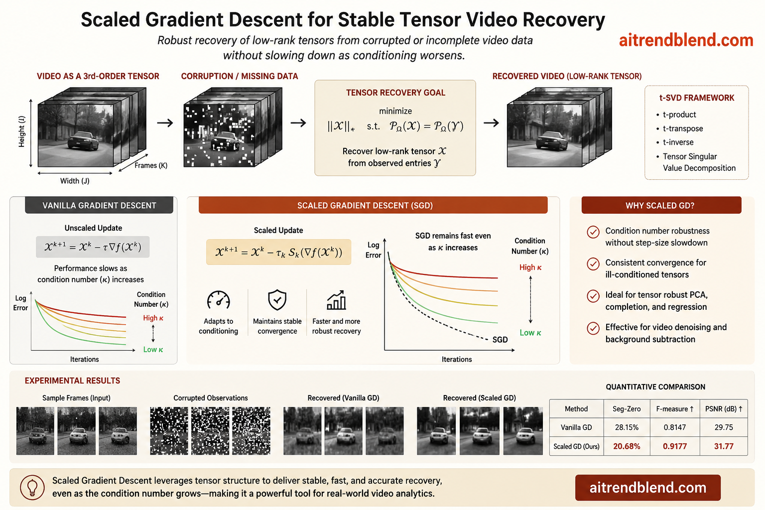
- The headline theoretical result is that ScaledGD converges at a constant linear rate regardless of the condition number of the true tensor, something plain gradient descent cannot promise.
- One algorithm, four jobs. The paper works out tensor robust PCA, tensor completion, robust tensor completion, and tensor regression, each with its own sample size and corruption threshold.
- On real video, ScaledGD with a Fourier transform beats or matches slower baselines on the Carphone and Coastguard sequences, and it wins on F measure for six of nine clips in a background subtraction benchmark.
- The catch, which the paper is upfront about, is that several tuning parameters still assume knowledge you would not have on a fresh, unlabeled video feed.
Why condition number keeps breaking gradient descent
Every low rank recovery method eventually runs into the same wall. You factor your target matrix or tensor as a product of two smaller pieces, say L times R transpose, and then chase the factors with gradient steps until the product matches your data. The trouble is that plain gradient descent moves at a speed set by the worst singular value ratio in the true object, what everyone calls the condition number, written kappa. A well behaved scene with kappa near one converges quickly. A scene with a dominant background and a much weaker secondary structure, kappa in the tens or higher, can make vanilla gradient descent crawl, and in some regimes it stalls out entirely before reaching an accurate answer.
This is not an academic footnote for anyone doing frame level video work. Lighting changes, shadows, camera noise, and compression artifacts all reshape the effective condition number of a video tensor from one clip to the next. A pipeline tuned on one sequence can quietly underperform on the next unless someone reruns a learning rate search, which does not scale if you are processing thousands of clips.
The matrix version of this problem already has an answer. Tong et al. showed in 2021 that preconditioning the gradient step by the inverse of a small Gram matrix, the method called scaled gradient descent, removes the dependence on the condition number for matrix recovery. Wu’s contribution is carrying that idea over to genuinely tensor structured data through the t-SVD, rather than flattening a video cube into a matrix and throwing away the temporal structure, or falling back on a Tucker decomposition that the paper shows performs noticeably worse on this kind of data.
The t-product, briefly
The t-SVD framework treats an order three tensor as a matrix whose entries are themselves short vectors along the third mode, then defines a product, called the t-product, using any invertible linear transform along that third mode. The discrete Fourier transform is the most familiar choice, which is why you will see ScaledGD DFT in the results tables, but the paper deliberately proves its guarantees for any invertible transform satisfying a mild orthogonality condition, and it also runs everything a second time with the discrete cosine transform to check that the theory is not secretly tied to Fourier structure.
Once you have a t-product, you can define a tensor version of the singular value decomposition, a tensor tubal rank, and a tensor nuclear norm, all of which behave enough like their matrix counterparts that convergence proofs carry over with real, if substantial, extra work. The paper is honest about this extra work. Its authors note that every matrix style inequality from the earlier scaled gradient papers had to be reproved using t-product properties rather than assumed by analogy.
What ScaledGD actually updates
Factor the target tensor as X equals L t-product R conjugate transpose, with L and R much smaller than the ambient tensor. Standard gradient descent nudges L and R by the raw gradient. ScaledGD instead multiplies each gradient by the inverse of a small r by r by n3 Gram tensor before taking the step, where r is the target rank and n3 is the number of frames or the third mode dimension.
That inverse is cheap because the Gram tensor lives in the small rank dimension, not the full frame size, so ScaledGD adds only a modest per iteration cost on top of ordinary gradient descent. The paper works out the flop count explicitly, arriving at roughly \(O(n_1 n_2 n_3 r + n_1 n_2 n_3 \log n_3)\) per step for a Fourier transform, dominated by the same fast Fourier transform cost you would pay anyway.
What that preconditioning buys you shows up cleanly in the proof. The convergence rate the paper derives is \(1 – 0.6\eta\) per iteration for tensor robust PCA, a number with no kappa in it at all. Ordinary gradient descent, by contrast, has a rate that degrades linearly with kappa, which is exactly why the ill conditioned curves in the paper’s own experiments flatten out for vanilla gradient descent while ScaledGD keeps dropping.
One recipe, four recovery problems
The paper does not stop at a single clean setting. It works the same scaled update into four related recovery problems, each with a slightly different twist and its own theoretical guarantee.
- Tensor robust PCA. Split a fully observed but corrupted tensor into a low rank part and a sparse outlier part, alternating a soft threshold step for the sparse component with the scaled gradient step for the low rank factors. This is the version used for video denoising.
- Tensor completion. Recover a low rank tensor from a random subset of its entries, adding a projection step that keeps the iterates from drifting toward incoherent, spiky solutions that would otherwise blow up the sample complexity.
- Robust tensor completion. The hardest of the four, combining partial observation with sparse corruption at the same time, which is closer to what a real surveillance feed looks like once you account for dropped frames and sensor glitches together.
- Tensor regression. Recover a low rank tensor from linear measurements rather than direct entries, relevant to compressed sensing style acquisition.
Each variant comes with its own sample complexity bound and, for the two robust problems, a maximum tolerable fraction of corrupted entries. The tensor completion bound, for instance, requires the observation probability p to scale at least like mu times the sum rank divided by the ambient size, up to log factors, which mirrors the matrix completion literature almost exactly once you substitute in the tensor rank quantities.
Reading the guarantee honestly
The convergence rate is genuinely independent of the condition number. The initialization and threshold schedule needed to get there are not free. Both depend on quantities such as the true singular value gap and the incoherence parameter that you will not know on an unlabeled clip, which the paper itself flags as a reason its stated theorem should be read as a proof that good parameters exist, not a recipe for finding them automatically.
What the synthetic experiments actually show
Before touching real video, the paper runs a clean synthetic comparison. It builds tensors with condition number one, five, ten, and twenty, then tracks the relative reconstruction error of ScaledGD against vanilla gradient descent over a thousand iterations, for both the Fourier and cosine transforms, across all four recovery problems.
The pattern is consistent across every one of the eight panels the paper reports. At kappa equal to one, the two methods are close, sometimes with vanilla gradient descent winning on raw wall clock time because it skips the preconditioning step. As kappa climbs to twenty, vanilla gradient descent for tensor robust PCA and robust tensor completion simply stops making progress, with the relative error stuck above one in ten thousand, while ScaledGD keeps descending at essentially the same rate it had at kappa equal to one. For tensor completion and tensor regression, both methods eventually reach machine precision, but ScaledGD gets there in a fraction of the iterations once kappa grows.
The paper also runs a parameter sweep across the threshold schedule and the step size, and finds ScaledGD stays accurate across a fairly wide band of settings, which matters because it suggests the method is not fragile to the exact hyperparameters chosen, at least in the synthetic regime where the ground truth condition number is known in advance.
Video denoising, where the numbers get concrete
The real world section is where this stops being an abstract convergence argument and starts looking like something a video pipeline could actually use. The authors corrupt a fraction of pixels in every frame of the Carphone and Coastguard sequences from the YUV benchmark set, adding Gaussian noise on top, then compare seven methods, ScaledGD with the Fourier and cosine transforms, the earlier TRPCA baseline with both transforms, a Tucker decomposition version of ScaledGD, and the EAPT alternating projection method with both transforms.
| Method | Carphone PSNR, alpha 0.1 | Carphone time, seconds | Coastguard PSNR, alpha 0.1 | Coastguard time, seconds |
|---|---|---|---|---|
| TRPCA DFT | 30.26 | 185.47 | 31.32 | 164.15 |
| ScaledGD Tucker | 24.20 | 53.57 | 22.80 | 39.29 |
| EAPT DFT | 30.58 | 30.28 | 30.09 | 24.24 |
| ScaledGD DFT | 30.98 | 33.08 | 30.42 | 22.96 |
Two things stand out here that are easy to miss if you only read the paper’s headline claim of superior recovery. First, ScaledGD Tucker, the same scaled update but wrapped around a Tucker decomposition instead of t-SVD, trails everything else by roughly six decibels of PSNR on both clips. That is a large gap for what is supposedly the same optimization idea, and it is the paper’s strongest piece of evidence that t-SVD is doing real work here, not just providing a convenient proof technique. Second, ScaledGD does not universally win. On Coastguard, TRPCA DFT edges it out on PSNR by about a third of a decibel, and the paper is upfront that this comes at a real cost, TRPCA DFT takes roughly seven times as long because it computes a full t-SVD every iteration rather than the cheap factor updates ScaledGD relies on. Whether that tradeoff is worth it depends entirely on whether your pipeline is PSNR constrained or latency constrained, and the paper does not run a statistical test across multiple corruption seeds to say whether that third of a decibel gap on Coastguard is even distinguishable from noise.
Background subtraction across nine real sequences
The second real world test uses the Background Models Challenge dataset, nine surveillance style clips where the goal is to separate a mostly static background from moving foreground objects using precision, recall, and F measure. Here the picture is less one sided than the headline number suggests. ScaledGD Tucker actually posts the highest recall on most videos, meaning it flags more true foreground pixels, but at a heavy cost in precision, since its F measure trails badly, in one case scoring 0.03 against ScaledGD’s 0.43 on the same clip. ScaledGD with either transform wins outright on F measure for six of the nine sequences, is closely comparable to TRPCA on a seventh, and EAPT DCT, the fastest method in the comparison, still lags ScaledGD on F measure on most clips despite running in roughly half the time. TRPCA remains the running time bottleneck throughout, at least eight and a half times slower than ScaledGD on the video where the two are closest in accuracy.
What the tables leave out
None of the reported PSNR, RSE, precision, recall, or F measure numbers in either real world table come with an error bar, a standard deviation across seeds, or a significance test. Every comparison is a single run per method per sequence. That is standard practice in this corner of the optimization literature, but it means a reader should treat close numbers, like the Coastguard PSNR gap between ScaledGD and TRPCA, as suggestive rather than conclusive without rerunning the comparison.
Where this fits if you build video pipelines
If your team already leans on low rank tensor recovery for denoising, stabilization, or background modeling, the practical takeaway is narrower than the abstract makes it sound. Vanilla gradient descent is fine as long as your data stays reasonably well conditioned, which for clean, evenly lit footage it often does. The moment you deal with harder lighting, occlusion heavy scenes, or a mix of camera qualities in one dataset, the effective condition number rises and a fixed learning rate schedule tuned on easy footage starts to underperform quietly rather than failing loudly. ScaledGD trades a small amount of per iteration overhead, one extra tensor inverse per factor per step, for insurance against that failure mode, without requiring you to know the condition number ahead of time to pick a working step size.
It is also worth noting where the method sits relative to newer video segmentation architectures, an area the site has covered before through frameworks like DVIS++ and Seg-Zero, which is one PLACEHOLDER link away in the video segmentation architecture comparison. Those methods learn a segmentation function directly through a neural network trained end to end. ScaledGD is a different animal entirely, an unsupervised, model based recovery procedure with a convergence proof, no labeled training data, and no learned parameters beyond the target rank and a handful of tuning constants. The two approaches are not competitors so much as tools for different stages of a pipeline, tensor recovery as a cheap, interpretable preprocessing step before or alongside a learned segmentation model, rather than a replacement for one.
Takeaway one
The condition number independence is the real contribution here, not the raw accuracy numbers, which are close to several existing baselines. If your video data has a wide range of effective conditioning across clips, that stability is worth more in practice than a fraction of a decibel of PSNR on any single sequence.
Takeaway two
The Tucker decomposition comparison is arguably the most useful negative result in the paper. Two optimizers with the same convergence proof template diverge by six decibels of PSNR purely because of which tensor decomposition they factor through, a reminder that the choice of tensor model matters as much as the choice of optimizer wrapped around it.
Limitations worth sitting with
The paper is candid about several gaps, and it is worth listing them plainly rather than glossing over them.
- The threshold schedule for the sparse component and the projection radius for tensor completion both depend on the true singular value gap and incoherence parameter of the unknown tensor, quantities you do not have access to on a fresh video feed. The theorem is explicitly framed as a proof that good parameters exist, not a way to find them.
- Every real world comparison is a single run, with no repeated trials, no confidence intervals, and no significance testing between close results such as the Coastguard PSNR gap.
- The theory covers order three tensors only. The authors state plainly that extending the guarantees to higher order tensors, which would matter for multichannel or multi camera video, is future work rather than something this paper delivers.
- The choice between the Fourier and cosine transforms is treated as a hyperparameter tried both ways rather than learned or selected automatically, and the paper says as much, calling the choice of transform an open problem.
- Tensor completion in this paper targets the Frobenius norm of the recovered tensor, not an entrywise error bound, so pixel level worst case guarantees are not covered here even though they would matter for artifact free video output.
The PyTorch implementation
The block below implements the t-product, t-transpose, and t-inverse operations under a discrete Fourier transform, a t-SVD routine built on batched SVD in the frequency domain, and the full ScaledGD update for tensor robust PCA from Algorithm 1 in the paper. A smoke test generates a synthetic low rank tensor corrupted with sparse outliers, runs the optimizer, and checks that the recovery error drops below a tight threshold.
import torch

torch.manual_seed(0)

def t_product(A, B):
    Af = torch.fft.fft(A, dim=2)
    Bf = torch.fft.fft(B, dim=2)
    Cf = torch.einsum('ijk,jlk->ilk', Af, Bf)
    C = torch.fft.ifft(Cf, dim=2).real
    return C

def t_transpose(A):
    Af = torch.fft.fft(A, dim=2)
    Ahf = Af.conj().permute(1, 0, 2)
    Ah = torch.fft.ifft(Ahf, dim=2).real
    return Ah

def t_inverse(A):
    Af = torch.fft.fft(A, dim=2).permute(2, 0, 1)
    Bf = torch.linalg.inv(Af).permute(1, 2, 0)
    B = torch.fft.ifft(Bf, dim=2).real
    return B

def t_svd(X, r):
    Xf = torch.fft.fft(X, dim=2).permute(2, 0, 1)
    U, S, Vh = torch.linalg.svd(Xf, full_matrices=False)
    U = U[:, :, :r].permute(1, 2, 0)
    S = S[:, :r]
    Vh = Vh[:, :r, :].permute(1, 2, 0)
    n3 = X.shape[2]
    Gf = torch.zeros(r, r, n3, dtype=torch.cfloat)
    for k in range(n3):
        Gf[:, :, k] = torch.diag(S[k, :].to(torch.cfloat))
    U = torch.fft.ifft(U, dim=2).real
    V = torch.fft.ifft(Vh.conj().permute(1, 0, 2), dim=2).real
    G = torch.fft.ifft(Gf, dim=2).real
    return U, G, V

def soft_threshold(M, zeta):
    return torch.sign(M) * torch.clamp(M.abs() - zeta, min=0.0)

def rpca_loss(L, R, S, Y):
    """f(F, S) = 0.5 * || L *_phi R^H + S - Y ||_F^2, matching Eq. 12 in the paper."""
    resid = t_product(L, t_transpose(R)) + S - Y
    return 0.5 * (resid ** 2).sum()

def evaluate(X_hat, X_star):
    """Relative Frobenius error and PSNR, the two metrics used in Table 1 of the paper."""
    rel_err = (X_hat - X_star).norm() / X_star.norm()
    mse = ((X_hat - X_star) ** 2).mean()
    peak = X_star.abs().max()
    psnr = 20 * torch.log10(peak) - 10 * torch.log10(mse)
    return rel_err.item(), psnr.item()

class ScaledGDTensorRPCA:
    """ScaledGD for tensor robust PCA under t-SVD (DFT transform), Algorithm 1."""

    def __init__(self, rank, eta=0.5, zeta0=0.5, rho=0.95):
        self.r = rank
        self.eta = eta
        self.zeta0 = zeta0
        self.rho = rho

    def fit(self, Y, num_iters=200):
        zeta = self.zeta0 * Y.abs().max()
        S = soft_threshold(Y, zeta)
        U, G, V = t_svd(Y - S, self.r)
        Ghalf = self._t_sqrt(G)
        L = t_product(U, Ghalf)
        R = t_product(V, Ghalf)
        history = []
        for t in range(num_iters):
            S = soft_threshold(Y - t_product(L, t_transpose(R)), zeta)
            RtR_inv = t_inverse(t_product(t_transpose(R), R))
            LtL_inv = t_inverse(t_product(t_transpose(L), L))
            err = t_product(L, t_transpose(R)) + S - Y
            L_new = L - self.eta * t_product(t_product(err, R), RtR_inv)
            R_new = R - self.eta * t_product(t_product(t_transpose(err), L), LtL_inv)
            L, R = L_new, R_new
            zeta = self.rho * zeta
            history.append(err.norm().item())
        return L, R, S, history

    @staticmethod
    def _t_sqrt(G):
        Gf = torch.fft.fft(G, dim=2).permute(2, 0, 1)
        eigval, eigvec = torch.linalg.eigh(Gf)
        eigval = torch.clamp(eigval, min=0.0)
        sqrt_eigval = torch.sqrt(eigval)
        Gsqrt_f = eigvec @ torch.diag_embed(sqrt_eigval.to(torch.cfloat)) @ eigvec.conj().transpose(-2, -1)
        Gsqrt_f = Gsqrt_f.permute(1, 2, 0)
        return torch.fft.ifft(Gsqrt_f, dim=2).real


def smoke_test():
    n1, n2, n3, r = 20, 18, 6, 3
    Ustar = torch.randn(n1, r, n3)
    Vstar = torch.randn(n2, r, n3)
    Xstar = t_product(Ustar, t_transpose(Vstar))
    Xstar = Xstar / Xstar.norm() * (n1 * n2 * n3) ** 0.5

    S_star = torch.zeros(n1, n2, n3)
    mask = torch.rand(n1, n2, n3) < 0.1
    S_star[mask] = torch.randn(mask.sum().item()) * Xstar.abs().mean() * 3

    Y = Xstar + S_star

    model = ScaledGDTensorRPCA(rank=r, eta=0.5, zeta0=0.5, rho=0.95)
    L, R, S_hat, history = model.fit(Y, num_iters=150)

    X_hat = t_product(L, t_transpose(R))
    final_loss = rpca_loss(L, R, S_hat, Y)
    rel_err, psnr = evaluate(X_hat, Xstar)
    print("initial residual norm:", history[0])
    print("final residual norm:", history[-1])
    print("final objective value:", final_loss.item())
    print("final relative recovery error:", rel_err)
    print("final PSNR (dB):", psnr)
    assert history[-1] < history[0], "ScaledGD did not reduce the residual"
    assert rel_err < 0.05, "ScaledGD did not recover the low rank tensor accurately"
    print("smoke test passed")

if __name__ == "__main__":
    smoke_test()
Conclusion
Strip away the appendix full of concentration inequalities and what this paper delivers is a fairly specific, fairly useful claim. If you are recovering a low rank tensor from corrupted or incomplete video data, preconditioning your gradient steps by a small tensor inverse removes the single biggest source of unpredictable slowdown, namely how well conditioned your particular clip happens to be, and it does so without the expensive full t-SVD computation that older robust PCA solvers rely on every iteration.
The conceptual shift is smaller than it might sound but still matters. Scaled gradient descent for matrices was already known to break the condition number dependence. What Wu’s analysis establishes is that the same preconditioning idea survives the jump from matrices to the t-SVD tensor algebra almost intact, provided you are willing to redo every supporting inequality in tensor form, which the appendix spends dozens of pages doing. That is not a flashy result, but it is the kind of foundational work that later applied papers tend to quietly depend on.
Where this could travel next is fairly clear from the paper’s own future directions section. Learning the threshold schedule automatically through deep unfolding, rather than hand tuning it against an unknown ground truth, would remove the biggest practical obstacle to using this in an unsupervised pipeline. Extending the guarantees past order three tensors would open the door to multi camera or multispectral video, where a third mode alone cannot capture every axis of correlation in the data.
The honest limitations do not undercut the contribution so much as scope it correctly. This is a tool for the specific situation where you know or can estimate your target rank, where your corruption or missing data pattern is reasonably close to the sparse or random models the theory assumes, and where you care more about a stable, predictable convergence rate than squeezing out the last fraction of a decibel against a slower, fully converged baseline.
For teams building video preprocessing or background modeling components, the practical message is simple. Stop tuning a fixed learning rate against your best behaved test clip and hoping it generalizes. A scaled update costs one small tensor inverse per iteration and buys you a convergence rate that does not care how badly conditioned your worst clip turns out to be.
Frequently asked questions
What problem does ScaledGD solve that ordinary gradient descent does not?
Ordinary gradient descent for low rank tensor recovery slows down, and in ill conditioned cases stalls entirely, as the ratio between the largest and smallest relevant singular values of the true tensor grows. ScaledGD preconditions each gradient step by a small tensor inverse, which the paper proves removes that dependence, giving a constant convergence rate no matter how poorly conditioned the target tensor is.
Does this replace learned video segmentation models?
No. ScaledGD is an unsupervised, model based recovery method with a convergence proof and no trainable parameters beyond the target rank and a few tuning constants. It works well as a preprocessing or denoising step, separate from learned segmentation architectures that are trained end to end on labeled data.
Why does the Tucker decomposition version perform so much worse?
The paper’s own comparison shows ScaledGD built on a Tucker decomposition trailing the t-SVD version by roughly six decibels of PSNR on both video sequences tested. The authors attribute this to t-SVD providing a more realistic model of how correlation across video frames is structured, compared to the more generic multilinear structure Tucker decomposition assumes.
Is the Fourier transform required for this method to work?
No. The theory is proved for any invertible linear transform satisfying a mild orthogonality condition. The paper runs every experiment with both the discrete Fourier transform and the discrete cosine transform, and results are broadly similar between the two, though the paper itself calls the choice of which transform to use an open problem rather than a solved one.
Do I need to know the rank of my video tensor in advance?
Yes, the target tubal rank r is a required input to every variant of the algorithm, along with a threshold schedule for the sparse component in the robust PCA and robust completion settings. The paper treats learning these automatically as future work rather than something the current method handles.
How much slower is ScaledGD than vanilla gradient descent per iteration?
The extra cost is one tensor inverse of a small r by r by n3 tensor per factor per iteration, which the paper shows is dominated by the same fast Fourier transform cost the method already pays, so the per iteration overhead is modest even though the accuracy and stability gains, especially under high condition number, are substantial.
Read the full paper for the complete convergence proofs and appendix derivations.
Read the paper on JMLR View the code repositoryWu, T. (2026). Guaranteed nonconvex low rank tensor estimation via scaled gradient descent. Journal of Machine Learning Research, 27, 1 to 90. Available at jmlr.org/papers/v27/25-0012.html.
This analysis is based on the published paper and an independent evaluation of its claims.