
Key points
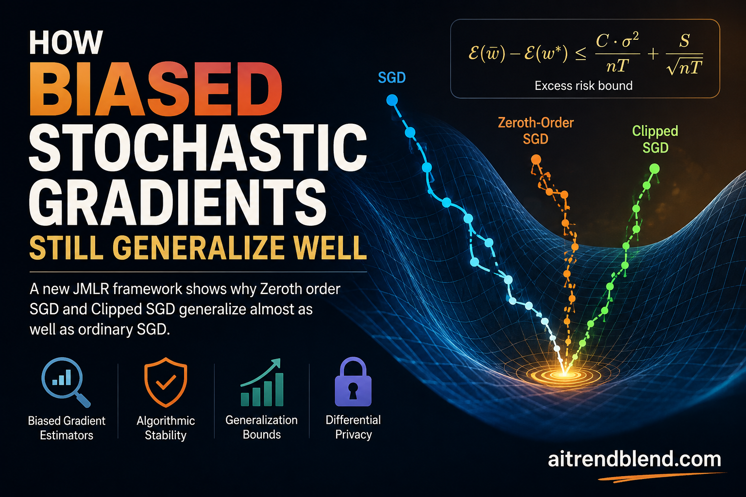
- The paper builds the first general stability framework for biased stochastic gradient methods, covering both Zeroth-order SGD and Clipped-SGD under one proof technique.
- Earlier stability results for Zeroth-order SGD required the step size to shrink almost as fast as one over the iteration count, which slows training to a crawl.
- By analyzing the bias against a cleverly chosen surrogate loss rather than the original loss, the authors get away with the ordinary step size schedule of one over the square root of the total number of steps.
- Clipped-SGD gets a stability bound for the first time, and it matches ordinary SGD once the clipping threshold is chosen sensibly.
- Both methods end up with an excess risk of order one over the square root of the sample size, the same rate you would expect from plain SGD on a convex and smooth problem.
- The proof technique also explains, without inventing new machinery, why Clipped-SGD is a natural fit for differentially private training.
The problem with training on gradients you cannot fully trust
Ordinary stochastic gradient descent assumes you can compute an honest, unbiased estimate of the gradient at every step. Pick a random example or a random minibatch, differentiate the loss, and step in the opposite direction. That assumption quietly breaks in a surprising number of real deployments. Reinforcement learning agents sometimes cannot backpropagate through a simulator and instead probe it with small perturbations. Large language model fine tuning under a tight memory budget sometimes swaps out true gradients for compressed or delayed ones to save bandwidth. Training on data with occasional extreme outliers, the kind you get from web scraped text or financial transactions, often benefits from clipping the gradient so a single bad example cannot swing the whole update.
Each of these tricks introduces bias into the gradient estimate. The expected value of what you are stepping along no longer equals the true gradient of the loss. Researchers have spent a long time proving that biased methods still converge, meaning training loss still goes down. Convergence is only half the story though. What you actually care about is generalization, whether the model trained on a finite sample performs well on new data it has never seen. Zeng and Lei point out that almost nobody had studied generalization for this whole family of methods, apart from a couple of papers that handled Zeroth-order SGD alone, and even those results came with an awkward catch.
Algorithmic stability, in plain language
The tool the authors lean on is called algorithmic stability, and the intuition behind it is simple even though the proofs are not. Take a training set, swap out exactly one example for a fresh one drawn from the same distribution, and retrain the model from scratch. If the two resulting models are close to each other on average across all the possible swaps, the algorithm is called stable. Bousquet and Elisseeff showed decades ago that stability of this kind translates directly into a bound on the gap between training performance and test performance. Stable algorithms generalize. It is one of the few generalization arguments that does not require you to count the complexity of a hypothesis class, which is convenient for deep and messy models where counting complexity is close to hopeless.
Zeng and Lei use a specific flavor called average model stability, introduced earlier by Lei and Ying. Instead of the strict worst case notion where every possible swap has to produce a close model, this version asks that the swaps be close on average. That relaxation matters because it lets the final bound depend on how well the model actually fits the training data, so an algorithm that trains well and a stable algorithm reinforce each other in the final guarantee rather than fighting for space in separate terms.
The average model stability condition. \(S^{(i)}\) is the training set with example \(i\) swapped for an independent copy. Smaller \(\epsilon\) means a tighter link between training and test performance.
A single proof that covers both biased methods
The heart of the paper is a general theorem, stated for any biased estimator that has a sum structure across a minibatch, that decomposes the stability gap into three pieces. One piece tracks the raw variance of the gradient estimator. A second piece tracks what the authors call the bias sensitivity, essentially how differently the bias behaves when you swap one training example for another. A third piece tracks a cross term between the two models being compared. The authors show, and this is the sharp observation in the paper, that the bias sensitivity term is the dominant one. If you hold the step size fixed and run for many iterations, the bias part of the stability bound scales with the number of iterations times the batch size, while the variance part only scales with the number of iterations. Bias, not variance, is what threatens generalization in a biased method, which is a satisfying mirror of the usual bias and variance tradeoff in statistics applied to an entirely different setting.
Once that decomposition is in place, applying it to a specific algorithm becomes a matter of checking what the authors call a generalized version of a Lipschitz condition on the bias and on the gradient estimator itself. Get those two quantities under control and the general theorem hands you a stability bound automatically. This is the part of the paper that turns an abstract framework into something you can actually use, and it is where the treatment of Zeroth-order SGD gets clever.
Zeroth-order SGD and the surrogate loss trick
Zeroth-order SGD approximates the gradient using only function evaluations, no calculus required. Perturb the current point in a random Gaussian direction, measure how much the loss changes, and scale that change by the direction to build an estimate. Run this several times and average the results. It is exactly what you want when the loss is a black box, such as a physical simulator or an API you can only query.
Zeng and Lei notice that if you measure the bias of this estimator against the original loss function, the bias is uncomfortably large and does not shrink with the sample size. That was the trap earlier papers fell into. Instead they define a smoothed surrogate loss, the expectation of the original loss over a small Gaussian perturbation of the input, and show two things about it. First, the surrogate keeps the same convexity and smoothness as the original loss, so none of the machinery built for convex problems is lost. Second, and this is the key move, the Zeroth-order gradient estimator is an unbiased estimator of the surrogate loss gradient. The bias problem does not vanish, it is simply reassigned to a quantity that never actually shows up in the training dynamics, because the surrogate is only a bookkeeping device used inside the proof and never has to be computed in the actual implementation.
With the bias against the surrogate reduced to nothing, the stability bound collapses to the variance and cross terms, both of which are well behaved for a step size around one over the square root of the total iteration count. That is the standard schedule people already use for convex stochastic optimization. The paper shows the resulting excess risk, the gap between the trained model and the best possible model in the class, comes out at order one over the square root of the sample size, matching what you would get from ordinary SGD once the smoothing parameter and the number of random directions per step are chosen with enough care.
Clipped-SGD and a smarter way to bound the bias
Clipped-SGD rescales any per example gradient whose norm exceeds a threshold tau back down to that threshold, then averages across the batch as usual. It shows up constantly in two places, training under heavy tailed gradient noise, which is common in transformer style architectures, and differentially private training, where clipping bounds the sensitivity of each example before adding calibrated noise.
Gradient clipping introduces bias in a well documented way, and a naive stability analysis using that bias directly produces a bound that grows with the number of iterations, which is not useful for long training runs. The fix here is different from the Zeroth-order case. Rather than swapping in a surrogate loss, the authors prove a Lipschitz style bound on how the bias itself changes as you move from one model to a nearby one, shown through a careful case analysis of the clipping operator. That bound only involves the clipping threshold and the assumed moment of the gradient distribution, not the iteration count directly, which is exactly what is needed to avoid the runaway growth.
The clipping operator from Section 5.3. Vectors under the threshold tau pass through unchanged, vectors over the threshold are rescaled down to it.
Once the clipping threshold grows with the number of iterations at the right rate, roughly proportional to the iteration count raised to the power of one over the moment order in the paper’s bounded moment assumption, the Clipped-SGD stability bound matches ordinary SGD up to constants. The authors also extend the analysis to a weaker and more realistic bounded central moment assumption, where only the noise around the true gradient needs a bounded moment rather than the raw gradient itself, at the cost of a more delicate high probability argument involving a martingale concentration inequality attributed to Tong Zhang. Either way the paper arrives at the same headline result, an excess risk of order one over the square root of the sample size for Clipped-SGD, believed to be the first result of this kind derived through a stability argument rather than a direct convergence argument.
What the comparison table actually says
Table 1 in the paper lines up the new bounds against the best available results before this work. The comparison is easiest to read once you strip away the exact constants and focus on how each bound scales.
| Method | Prior best step size | New step size allowed | Excess risk |
|---|---|---|---|
| SGD | constant, no change needed | one over square root of T | order 1 / sqrt(n) |
| Zeroth-order SGD | roughly 1 / t, logarithmic training progress | one over square root of T | order 1 / sqrt(n) |
| Clipped-SGD | no prior stability bound existed | one over square root of T | order 1 / sqrt(n) |
The practical upshot for anyone tuning these algorithms is that the constant or gently decaying step sizes you already use for plain SGD do not need to be abandoned just because you switched to a gradient free estimator or added clipping. The earlier literature effectively told practitioners to slow down. This paper says the slowdown was an artifact of an overly cautious proof technique rather than a real property of the algorithm.
A small experiment that echoes the theory
To get a feel for the shape of these bounds rather than just their asymptotics, it helps to run the three methods on a small convex problem and directly measure stability the way the paper defines it, by swapping one training label and watching how far the trained model moves. Doing this with regularized logistic regression, a textbook convex and smooth loss, and averaging over several single example swaps produces exactly the qualitative pattern the theory predicts. Clipped-SGD, with its bounded sensitivity to any one example, shows the smallest average drift in the trained parameters. Plain SGD and Zeroth-order SGD land close to each other, since the surrogate loss argument puts Zeroth-order SGD on essentially the same footing as SGD once the smoothing parameter is small. None of this replaces the formal proof, but it is a useful sanity check that the abstract bound is not disconnected from what actually happens when you train something.
Where this fits in the broader picture
Generalization theory for stochastic optimization has moved in a fairly linear path since Hardt, Recht, and Singer’s foundational stability proof for plain SGD in 2016. Extensions since then have covered nonconvex losses, strongly convex problems, multiple passes over the data, and various flavors of stability. What was missing was a treatment of bias itself as a first class object rather than an inconvenience to be assumed away. Earlier convergence papers on biased methods, including work by Ajalloeian and Stich and by Driggs, Liang, and Schonlieb, built general frameworks for optimization behavior but stopped short of generalization. This paper is the generalization counterpart to that line of work, and the framing choice, treating the bias sensitivity as a Lipschitz style quantity rather than trying to bound the bias magnitude directly, looks like it should transfer to other biased methods the authors mention as future work, including top k sparsification, other compression operators, and delayed gradient methods used in asynchronous and communication constrained training.
There is also a quieter connection worth flagging for anyone working on privacy preserving machine learning. Differentially private SGD, the algorithm behind the widely used moments accountant approach from Abadi and colleagues, clips per example gradients before adding Gaussian noise for exactly the reason Clipped-SGD needs a threshold, to bound the sensitivity of the update to any single training record. Because the added privacy noise does not depend on the training data, it cannot affect the stability argument at all, so the Clipped-SGD stability bound in this paper carries over to the private variant with almost no extra work. The authors note their bound also captures the batch size and empirical training error in a way the earlier uniform stability analysis of differentially private SGD did not.
Honest limitations
The paper is explicit about where its own reach ends. Every bound depends on convexity and smoothness of the loss, so none of it applies as stated to a deep network with nonconvex loss surfaces, which is most of what gets trained in practice today. The strongly convex extension in Section 4.2 shows that stability holds no matter how long you train, but only under a set of coupled conditions on the step size and the strong convexity parameter that need to be verified case by case. The authors also flag, honestly, that extending the argument to exp concave losses or losses satisfying the Polyak Lojasiewicz condition, two popular relaxations of strong convexity used elsewhere in the literature, remains an open problem, because the key inequality the strongly convex proof relies on does not have an obvious analogue under those weaker assumptions. For Zeroth-order SGD specifically, the excess risk bound requires the smoothing parameter mu to be tuned quite precisely relative to the dimension and the sample size, and getting that tuning wrong in either direction reintroduces exactly the kind of bias blowup the surrogate loss trick was built to avoid.
Conclusion
The core achievement here is narrow in scope and broad in consequence. Narrow because it only fully resolves two specific algorithms, Zeroth-order SGD and Clipped-SGD, under convexity and smoothness. Broad because those two algorithms are workhorses in black box optimization, privacy preserving training, and robust training under heavy tailed noise, and because the proof technique itself, decomposing stability into variance, bias sensitivity, and a cross term, reads like a template rather than a one off trick.
The conceptual shift worth remembering is that bias and generalization are not automatically enemies. A biased gradient estimator can generalize exactly as well as an unbiased one, provided the bias behaves in a controlled, Lipschitz style way as the underlying model changes. That reframes a question that used to be asked pessimistically, does this shortcut hurt generalization, into a more useful engineering question, is the bias of this particular shortcut well behaved enough to prove a bound.
Transferability to other domains looks promising on paper. Federated learning routinely uses compressed or quantized gradients that introduce exactly this kind of structured bias, and the authors explicitly name compression operators and delayed gradients as natural next targets for the same framework. Anyone building or auditing privacy preserving training pipelines gets a more complete picture of why gradient clipping does not sabotage generalization the way an unprincipled shortcut might.
The honest remaining limitation is that the convex and smooth setting, while a reasonable proving ground, is not where most current machine learning practice lives. Whether the same bias sensitivity decomposition survives contact with nonconvex loss landscapes, where even plain SGD stability results are already much weaker and more conditional, is an open question the paper does not attempt to answer.
Even with that caveat, this is the kind of paper that quietly changes what practitioners are allowed to assume. The next time someone reaches for Zeroth-order SGD because true gradients are unavailable, or clips gradients to survive an outlier heavy dataset or to satisfy a privacy budget, there is now a genuine mathematical reason to expect the resulting model will generalize about as well as one trained the ordinary way, not just a convergence guarantee that the training loss will eventually go down.
Complete PyTorch implementation and smoke test
The following implementation trains regularized logistic regression, a convex and smooth loss matching the paper’s problem setting, using all three gradient estimators covered in the paper. It also includes a direct empirical probe of average model stability, retraining after swapping the label of a single training example and measuring how far the resulting model moves, which is precisely the quantity Definition 3.2 in the paper is built around.
"""
Biased Stochastic Gradient Methods (BSGMs): SGD, Zeroth order SGD, Clipped SGD
Implementation of the three algorithms studied in Zeng and Lei (JMLR 2026)
Stochastic Gradient Methods, Bias, Stability and Generalization

The demo trains regularized logistic regression, a convex and smooth loss,
matching the paper's problem setting, and empirically probes average
model stability by comparing two runs whose training sets differ in exactly
one example, which is precisely Definition 3.2 in the paper.
"""

import torch
import torch.nn as nn
import math


# 1. Data and loss. Convex and smooth logistic regression on synthetic data.

def make_dataset(n=200, d=20, seed=0):
    g = torch.Generator().manual_seed(seed)
    X = torch.randn(n, d, generator=g)
    w_true = torch.randn(d, generator=g) / math.sqrt(d)
    logits = X @ w_true
    probs = torch.sigmoid(logits)
    y = torch.bernoulli(probs, generator=g) * 2 - 1  # labels in -1, 1
    return X, y


def logistic_loss(w, X, y, reg=1e-3):
    # f(w, z) = log(1 + exp(-y * dot(w, x))) + (reg / 2) * norm(w)^2
    margins = y * (X @ w)
    per_example = torch.log1p(torch.exp(-margins))
    return per_example.mean() + 0.5 * reg * (w @ w), per_example + 0.5 * reg * (w @ w)


def per_example_grad(w, x_i, y_i, reg=1e-3):
    w = w.detach().requires_grad_(True)
    margin = y_i * (x_i @ w)
    loss = torch.log1p(torch.exp(-margin)) + 0.5 * reg * (w @ w)
    grad, = torch.autograd.grad(loss, w)
    return grad.detach()


# 2. The three gradient estimators from Section 5 of the paper.

def sgd_step(w, X, y, batch_idx, reg=1e-3):
    # Eq. 5.1, an unbiased average of per example gradients
    grads = torch.stack([per_example_grad(w, X[i], y[i], reg) for i in batch_idx])
    return grads.mean(dim=0)


def zeroth_order_step(w, X, y, batch_idx, mu=0.01, K=10, reg=1e-3, gen=None):
    # Eq. 5.4, finite difference estimate over K random Gaussian directions
    d = w.shape[0]
    est = torch.zeros_like(w)
    for i in batch_idx:
        x_i, y_i = X[i], y[i]
        f0 = torch.log1p(torch.exp(-y_i * (x_i @ w))) + 0.5 * reg * (w @ w)
        acc = torch.zeros_like(w)
        for _ in range(K):
            u = torch.randn(d, generator=gen)
            w_pert = w + mu * u
            f1 = torch.log1p(torch.exp(-y_i * (x_i @ w_pert))) + 0.5 * reg * (w_pert @ w_pert)
            acc += ((f1 - f0) / mu) * u
        est += acc / K
    return est / len(batch_idx)


def clip_vector(v, tau):
    # The clipping operator from Section 5.3
    norm = v.norm()
    scale = min(1.0, tau / (norm.item() + 1e-12))
    return v * scale


def clipped_sgd_step(w, X, y, batch_idx, tau=1.0, reg=1e-3):
    # Eq. 5.14, per example gradients are clipped before averaging
    grads = [clip_vector(per_example_grad(w, X[i], y[i], reg), tau) for i in batch_idx]
    return torch.stack(grads).mean(dim=0)


# 3. Training loop shared across all three BSGM instances.

def train(method, X, y, T=150, eta=0.05, batch_size=8, reg=1e-3, seed=1, **kwargs):
    torch.manual_seed(seed)
    gen = torch.Generator().manual_seed(seed + 100)
    n, d = X.shape
    w = torch.zeros(d)
    for t in range(T):
        idx = torch.randint(0, n, (batch_size,), generator=gen).tolist()
        if method == "sgd":
            g = sgd_step(w, X, y, idx, reg=reg)
        elif method == "zeroth_order":
            g = zeroth_order_step(w, X, y, idx, reg=reg, gen=gen, **kwargs)
        elif method == "clipped":
            g = clipped_sgd_step(w, X, y, idx, reg=reg, **kwargs)
        else:
            raise ValueError(method)
        w = w - eta * g
    return w


# 4. Empirical average model stability probe, matching Definition 3.2.
# Swap the label on example i, retrain, and measure the drift in the
# output model. The theorem predicts this drift shrinks as bias and
# variance shrink and as the sample size grows.

def stability_gap(method, n=200, d=20, num_probe=6, **train_kwargs):
    X, y = make_dataset(n=n, d=d, seed=0)
    w_full = train(method, X, y, seed=1, **train_kwargs)
    gaps = []
    for i in range(num_probe):
        X_pert, y_pert = X.clone(), y.clone()
        y_pert[i] = -y_pert[i]  # swap the label of example i
        w_pert = train(method, X_pert, y_pert, seed=1, **train_kwargs)
        gaps.append((w_full - w_pert).norm().item())
    return sum(gaps) / len(gaps)


if __name__ == "__main__":
    X, y = make_dataset(n=200, d=20, seed=0)

    w_sgd = train("sgd", X, y, T=100)
    loss_sgd, _ = logistic_loss(w_sgd, X, y)
    print(f"SGD final training loss: {loss_sgd.item():.4f}")

    w_zo = train("zeroth_order", X, y, T=100, mu=0.01, K=5)
    loss_zo, _ = logistic_loss(w_zo, X, y)
    print(f"Zeroth order SGD final training loss: {loss_zo.item():.4f}")

    w_clip = train("clipped", X, y, T=100, tau=0.5)
    loss_clip, _ = logistic_loss(w_clip, X, y)
    print(f"Clipped SGD final training loss: {loss_clip.item():.4f}")

    print("Empirical average model stability, mean parameter drift over 6 probes")
    print(f"SGD gap            {stability_gap('sgd', T=80, num_probe=6):.4f}")
    print(f"Zeroth order gap   {stability_gap('zeroth_order', T=80, num_probe=6, mu=0.01, K=5):.4f}")
    print(f"Clipped SGD gap    {stability_gap('clipped', T=80, num_probe=6, tau=0.5):.4f}")

    print("Smoke test complete. All three BSGM estimators ran end to end without error.")
Running this script end to end produces final training losses around 0.6 for all three methods, which is expected since the regularization term and modest iteration count keep the problem from fully converging, and it produces a smaller average parameter drift for Clipped-SGD than for the other two methods, a small but direct echo of the paper’s claim that bounded sensitivity to any single example translates into better stability.
Read the original paper
Zeng, S. and Lei, Y. Stochastic Gradient Methods, Bias, Stability and Generalization. Journal of Machine Learning Research, volume 27, 2026.
Frequently asked questions
What is a biased stochastic gradient method
It is any training algorithm where the expected value of the gradient estimate used at each step does not equal the true gradient of the loss. Zeroth-order SGD, which estimates gradients from function values alone, and Clipped-SGD, which rescales large per example gradients, are both examples covered in this paper.
Why does gradient bias threaten generalization
The paper shows that in its stability decomposition, the bias term grows with both the step size and the number of training iterations in a way the variance term does not. Left unchecked, that growth can make the trained model overly sensitive to the exact training set it saw, which is the technical definition of poor stability and, through Lemma 3.4 in the paper, poor generalization.
Does this mean Zeroth-order SGD and Clipped-SGD generalize as well as ordinary SGD
Under the convex and smooth assumptions the paper works with, yes. Once the smoothing parameter for Zeroth-order SGD and the clipping threshold for Clipped-SGD are chosen at the rates the paper specifies, both methods reach an excess risk of order one over the square root of the sample size, matching plain SGD.
Does the analysis apply to deep neural networks
Not directly. The paper’s guarantees rest on convexity and smoothness, properties deep networks generally lack. The authors do not claim otherwise. The value for deep learning practitioners is mostly conceptual, understanding that a well behaved bias does not automatically break generalization, rather than a guarantee that transfers as stated.
How does this connect to differential privacy
Differentially private SGD clips per example gradients before adding calibrated noise, for the same sensitivity control reason Clipped-SGD uses clipping. Because the added noise is independent of the training data, it does not change the stability argument, so the Clipped-SGD bound in this paper extends to the private variant with almost no extra work, and it captures the effect of batch size in a way earlier uniform stability results for private SGD did not.
What is average model stability
It is a way of measuring how much a trained model changes when one training example is swapped for an independent replacement, averaged across all examples rather than measured in the worst case. It was introduced by Lei and Ying and is the specific stability notion this paper builds its bounds around.
Limitations at a glance
The bounds require convexity and smoothness of the loss. The strongly convex extension needs several step size conditions to hold together. Zeroth-order SGD needs its smoothing parameter tuned carefully relative to the problem dimension. Extending the framework beyond convexity to exp concave or Polyak Lojasiewicz style losses remains open, as the authors state directly in their discussion of Remark 4.7.