
Key points
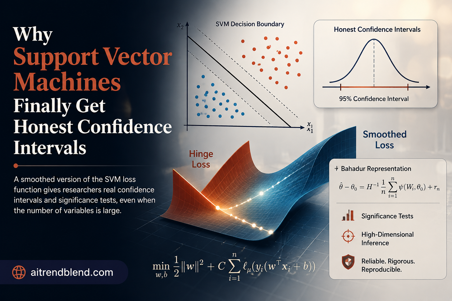
- The SVM decision boundary is described by parameters, and researchers have always wanted to test whether individual variables genuinely move that boundary.
- The standard hinge loss has a kink at zero, so it cannot be differentiated everywhere, which breaks the usual machinery for building confidence intervals.
- Rybak, Battey and Zhou replace the kink with a convolution smoothed version, producing a loss that is convex and twice differentiable everywhere.
- Their smoothed estimator keeps the same convergence rate as the classical SVM while needing a weaker condition on the number of variables for its confidence intervals to be trustworthy.
- Simulations in the paper show standard SVM confidence intervals collapsing toward zero coverage once the variable count climbs past about twenty, while the smoothed version holds close to the target the whole way.
- The paper also draws a direct line between the SVM’s implicit coefficients and the more familiar language of probability models such as logistic regression.
The problem nobody likes to admit about SVM coefficients
Support vector machines have been a workhorse of classification since Cortes and Vapnik introduced them in 1995. Feed the model a set of labeled examples and it finds a hyperplane that separates the classes with the widest possible margin. That hyperplane has a direction, described by a weight vector, and an offset, described by a bias term. Together they form a parameter vector that looks, on paper, exactly like a regression coefficient vector. Which raises an obvious question. If a weight on some gene expression variable comes out large and positive, does that mean the variable actually matters, or could a random dataset of the same size have produced a similarly large weight by chance alone?
Answering that question properly requires more than fitting the model once. It requires knowing the sampling distribution of the estimated weights, so you can build a confidence interval or run a formal significance test. For most models built on smooth, differentiable loss functions, that distribution follows from fairly standard asymptotic theory. The SVM refuses to cooperate, because its loss function, the hinge loss, is not differentiable at the one point that matters most, exactly where a prediction sits on the decision boundary. The empirical loss inherits that kink, and the usual proof techniques for building confidence sets simply do not apply cleanly.
Koo, Lee, Kim and Park worked out a solution back in 2008, deriving what is called a Bahadur representation for the plain SVM estimator, essentially a formula that approximates the estimation error as a sum of simple independent terms, which then lets you invoke a central limit theorem. It worked, but their own simulations hinted at a limitation. The approximation only behaved well when the sample size n was much larger than the number of candidate variables p. Once p grew to be a sizable fraction of n, the theoretical guarantees quietly stopped applying, right at the moment when researchers most want to know which of many candidate variables are real.
Why earlier attempts at smoothing did not fully solve it
The idea of softening the hinge loss is not new. Suykens and Vandewalle proposed replacing it with a squared loss back in 1999, which is mathematically equivalent to fitting a ridge regression against a binary target, a clever shortcut but one that changes what the estimator is actually targeting. Lee and Mangasarian took a more direct route in 2001, approximating the subgradient of the hinge loss with the cumulative distribution function of a logistic random variable, producing a loss that is smooth but was never given the finite sample statistical guarantees this new paper provides.
The closest prior attempt, and the one this paper spends the most time comparing itself against, comes from Wang, Yang, Chen and Liu in 2019. They borrowed a technique called Horowitz smoothing from the quantile regression literature, replacing a hard indicator function inside the hinge loss with a smooth cumulative distribution function estimate. It works, and it comes with real non asymptotic guarantees, but the resulting loss function is not globally convex. That matters in practice, because a non convex objective can have multiple local minima, and it complicates the theory needed to say precisely how many variables the method can tolerate before its confidence intervals start to misbehave.
What convolution smoothing actually does to the loss
Rybak, Battey and Zhou, working out of Imperial College London and the University of Illinois Chicago, take a cleaner route conceptually. Start from the observation that the hinge loss can be written as an integral against the empirical distribution of the margin residuals. Replace that empirical distribution with a version smoothed by a kernel, the same kind of kernel used in ordinary kernel density estimation, and the resulting loss becomes a convolution of the original hinge function with a smoothing kernel.
The population hinge loss the classical SVM minimizes, where Y is the class label and X is the feature vector.
The smoothed empirical loss the authors work with takes the form
The convolution smoothed hinge loss, where K is a symmetric kernel density and h is a bandwidth that shrinks toward zero as the sample grows.
As long as the kernel K is non negative, this loss is convex, and unlike Horowitz smoothing it stays convex globally rather than only locally. It is also twice continuously differentiable, which means its gradient and Hessian exist everywhere and can be written down explicitly.
The gradient and Hessian of the smoothed loss, where the bar over K denotes its cumulative distribution function.
One tidy result the authors prove early on is that choosing a logistic kernel recovers the Lee and Mangasarian smoothing exactly, up to a rescaling. So the older method turns out to be a special case of this broader convolution based family, rather than a separate idea. That reframing lets the paper inherit and extend, rather than compete with, decades of kernel smoothing theory borrowed from the quantile regression literature, particularly work by Fernandes, Guerre and Horta, and by He, Pan, Tan and Zhou.
Choosing a bandwidth is not cosmetic
The bandwidth h plays the same role here as it does in any kernel method, controlling a tradeoff between bias and variance. Set h close to zero and the smoothed loss converges back toward the original hinge loss, kink and all. Set h large and the loss becomes flatter and easier to optimize but drifts further from the quantity you actually care about. The paper works out precise rates. The bias introduced by smoothing scales like h squared, and there is a lower bound on how small h can be relative to the sample size and dimension for the finite sample bounds to hold. In the simulations, the authors settle on h equal to the fourth root of p over n, a rule that keeps the bandwidth shrinking as data accumulates but not so quickly that variance dominates in high dimensional settings.
The statistical guarantees, in plain terms
The heart of the paper is a pair of finite sample results. The first bounds how far the smoothed estimator can land from the true population minimizer, showing that the estimation error scales at the same rate, proportional to the square root of p over n, that the classical unpenalized SVM achieves. In other words, smoothing does not cost you anything in terms of raw accuracy.
The second and more consequential result is a Bahadur representation for the smoothed estimator, a formula approximating the scaled estimation error by a sum of independent terms plus a remainder that shrinks fast.
The Bahadur remainder bound. Minimizing this expression over the bandwidth h produces a convergence rate of p to the seven eighths power over n to the three eighths power.
Working through that minimization, the paper shows the distributional approximation for the smoothed SVM stays valid as long as p to the power seven thirds grows more slowly than n. Compare that with the condition required for the original unsmoothed SVM, or for the Horowitz smoothed version of Wang and colleagues, both of which need something closer to p cubed growing more slowly than n, up to logarithmic factors. That difference sounds abstract until you translate it into an example. Suppose your sample size is ten thousand. Under the older condition, the theory starts to break down somewhere around twenty two variables. Under the new condition, it holds comfortably out past two hundred variables. That is the practical payoff of insisting on a globally convex, twice differentiable loss rather than a merely smooth one.
Why this matters beyond the math
Most applied researchers reaching for an SVM are not thinking about differentiability. They want to know whether variable seven actually predicts the outcome or whether the model latched onto noise. This paper is the first to give that question a statistically honest answer that keeps working as the variable count grows, which is exactly the regime where genomics, text classification and sensor data problems tend to live.
What the simulations actually show
Theory is one thing. The authors back it up with simulations built on Gaussian class conditional densities, mirroring the setup Koo and colleagues used in 2008 so the comparison is apples to apples. Three results stand out.
First, they compare the size of the Bahadur remainder directly, the leftover error term that should shrink to nothing for the asymptotic theory to kick in. For the plain SVM, with the ratio of sample size to variable count fixed at fifty, the remainder grows steadily as both n and p increase together, ballooning past ten in some runs once p reaches five hundred. For the smoothed version under the identical setup, the remainder stays under two across the entire range. That is a large practical gap hiding behind what looks like a small change to the loss function.
Second, and probably most convincing for a working statistician, they measure Type 1 error rates for testing whether a genuinely irrelevant variable gets flagged as significant at the nominal five percent level. Here are the actual median rates reported in the paper across a grid of sample sizes and variable counts.
| Sample size n | Variables p | SVM Type 1 error | Smoothed SVM Type 1 error |
|---|---|---|---|
| 200 | 2 | 5% | 3% |
| 200 | 6 | 6% | 4% |
| 200 | 12 | 16% | 10% |
| 200 | 16 | 28% | 8% |
| 200 | 20 | 62% | 8% |
| 750 | 2 | 5% | 6% |
| 750 | 6 | 5% | 4% |
| 750 | 12 | 6% | 3% |
| 750 | 16 | 9% | 3% |
| 750 | 20 | 10% | 2% |
Look at the row for two hundred observations and twenty variables. The plain SVM flags a truly irrelevant variable as significant sixty two percent of the time, when it should only do so five percent of the time by construction. That is not a subtle miscalibration, it is a model telling you a coin flip’s worth of noise variables are real signal. The smoothed version, under the identical data, stays at eight percent, still a bit above nominal but in a completely different league.
Third, the paper checks coverage ratios directly, meaning how often a ninety five percent confidence interval actually contains the true coefficient across five hundred simulation runs with a fixed sample size of five hundred. The plain SVM’s coverage starts near the target around ninety five percent when there are only two variables, then slides steadily downward as more variables are added, dropping to roughly ten to twenty percent coverage by the time thirty variables are in play. The smoothed version barely moves off ninety five percent across that entire range.
Two ways to test a coefficient, and why the choice matters
Once you have a Bahadur representation, the natural next step is a Wald type test, the familiar approach of taking your estimated coefficient, dividing by its estimated standard error, and comparing against a normal distribution. The paper builds exactly that machinery. But it also offers a second option, a score based test, which evaluates the gradient of the smoothed loss directly at a hypothesized parameter value rather than at the fitted estimate.
The advantage of the score approach shows up in an edge case familiar to anyone who has run into Fieller’s problem from 1954, where the set of parameter values consistent with the data fails to form a clean interval, sometimes splitting into two disconnected pieces or even covering the entire real line. Wald based intervals cannot represent that possibility gracefully. Score based confidence sets, built by inverting a self normalized test statistic, can. The tradeoff is computational. A score test needs to be evaluated across a grid of candidate parameter values rather than computed once, so it costs more to run, and the paper is upfront about that cost rather than glossing over it.
From decision boundary back to probability
One of the more conceptually satisfying sections of the paper steps back from computation and asks what an SVM coefficient actually means. The population SVM, it turns out, is secretly estimating the Bayes classifier, the theoretically optimal decision rule based on the true conditional probability of belonging to each class. Once you restrict attention to linear decision boundaries, that fact implies the SVM’s coefficients are implicitly estimating parameters of what statisticians call a linear probability model, the same model discussed by Cox and Wermuth in 1992 and later by Battey, Cox and Jackson in 2019.
That connection has a genuinely useful consequence. The ratio of two SVM coefficients, weight on variable j divided by weight on variable k, has a direct interpretation as how much variable j would need to change to match the effect on the predicted probability of a one unit change in variable k. It is not identical to the corresponding ratio in a logistic regression, because the two models cannot both be exactly correct simultaneously, but the paper shows the estimated ratios under both models are targeting the same underlying quantity. That gives applied researchers permission to talk about SVM coefficients the way they already talk about regression coefficients, with an actual mathematical justification behind the comparison rather than a hand wave.
The nonlinear extension, briefly
For readers who care primarily about prediction rather than interpretation, the paper also extends convolution smoothing to kernel SVMs, the nonlinear cousins of the linear model that use functions such as radial basis kernels to draw curved decision boundaries. The same smoothing idea applies to the quadratic program Mangasarian described in 2000, producing a convex, twice differentiable objective there as well, though the authors are candid that this extension trades away the clean coefficient level interpretation that motivates most of the paper.
Honest limitations
The paper is careful about what it does and does not establish, and it is worth being equally careful summarizing it. The finite sample bounds depend on the feature vector being sub Gaussian, meaning its tails cannot be too heavy, an assumption that is reasonable for many engineered feature sets but not guaranteed for raw, unprocessed data with outliers. The theory also assumes the population SVM minimizer is unique, a condition that fails in genuinely degenerate cases where the classes overlap in specific structured ways. The simulations, while extensive, all use Gaussian class conditional densities with a shared covariance matrix, a convenient setting for deriving closed form population parameters but not necessarily representative of messier real world class distributions. Choosing the bandwidth in practice still requires the analyst to pick a rate, and while the paper shows robustness to different kernel choices in its appendix, it does not offer a fully automatic, data driven bandwidth selection rule the way some quantile regression methods do. Finally, this is a peer reviewed paper in the Journal of Machine Learning Research, which is a strong signal of rigor, but as with any single paper, independent replication on real datasets outside the simulation study would strengthen confidence in how the method behaves outside idealized settings.
A working implementation
The equations translate fairly directly into code. Below is a complete, runnable PyTorch implementation of the convolution smoothed SVM loss using a Gaussian kernel, along with a small training loop and a smoke test on synthetic data so you can see the smoothed loss actually train a linear classifier end to end.
import torch
import torch.nn as nn
import math

# Gaussian kernel convolution smoothed hinge loss
# Implements the loss from Rybak, Battey and Zhou, using the closed form
# integral of a Gaussian kernel against the positive part function.

class ConvSmoothedHingeLoss(nn.Module):
    def __init__(self, bandwidth=0.5):
        super().__init__()
        self.h = bandwidth

    def forward(self, margins):
        # margins is 1 minus y times the raw score, one entry per sample
        # For a Gaussian kernel the smoothed hinge loss has a closed form
        # using the standard normal pdf phi and cdf Phi.
        z = margins / self.h
        normal = torch.distributions.Normal(0.0, 1.0)
        phi = torch.exp(normal.log_prob(z))
        cap_phi = normal.cdf(z)
        loss_per_sample = margins * cap_phi + self.h * phi
        return loss_per_sample.mean()


class SmoothedLinearSVM(nn.Module):
    def __init__(self, num_features):
        super().__init__()
        self.linear = nn.Linear(num_features, 1, bias=True)

    def forward(self, x):
        return self.linear(x).squeeze(-1)


def train_smoothed_svm(x, y, epochs=300, lr=0.1, bandwidth=0.5, weight_decay=1e-3):
    model = SmoothedLinearSVM(x.shape[1])
    loss_fn = ConvSmoothedHingeLoss(bandwidth=bandwidth)
    optimizer = torch.optim.Adam(model.parameters(), lr=lr, weight_decay=weight_decay)

    for epoch in range(epochs):
        optimizer.zero_grad()
        scores = model(x)
        margins = 1.0 - y * scores
        loss = loss_fn(margins)
        loss.backward()
        optimizer.step()
        if (epoch + 1) % 50 == 0:
            print(f"epoch {epoch + 1} loss {loss.item():.4f}")

    return model


def evaluate(model, x, y):
    with torch.no_grad():
        scores = model(x)
        preds = torch.sign(scores)
        accuracy = (preds == y).float().mean().item()
    return accuracy


if __name__ == "__main__":
    # Smoke test on dummy data, two Gaussian blobs in ten dimensions
    torch.manual_seed(0)
    n_samples, n_features = 400, 10
    mean_pos = torch.ones(n_features) * 1.2
    mean_neg = -mean_pos

    x_pos = mean_pos + torch.randn(n_samples // 2, n_features)
    x_neg = mean_neg + torch.randn(n_samples // 2, n_features)
    x = torch.cat([x_pos, x_neg], dim=0)
    y = torch.cat([torch.ones(n_samples // 2), -torch.ones(n_samples // 2)])

    trained_model = train_smoothed_svm(x, y, epochs=300, bandwidth=0.5)
    acc = evaluate(trained_model, x, y)
    print(f"training accuracy {acc:.3f}")
    print("fitted weight vector", trained_model.linear.weight.detach())
Running that smoke test should print a shrinking loss over the three hundred epochs and finish with training accuracy well above ninety percent on the synthetic blobs, confirming the smoothed objective is doing its job as a working classifier before you ever get to the inference machinery layered on top of it.
Conclusion
The core achievement here is narrower than it might sound and more useful for it. The authors did not invent a new classifier. They took the exact same support vector machine researchers have used for three decades and asked a focused question, what happens to the statistical guarantees if you replace one kink in the loss function with a smooth curve. The answer turns out to matter a great deal once the number of candidate variables grows past a small handful, which describes most modern applications of the method.
The conceptual shift is subtle but important. Statisticians have long treated smoothing as primarily a computational convenience, a way to make optimization easier or gradients cheaper to compute. This paper reframes convolution smoothing as a statistical tool in its own right, one that changes the conditions under which inference is even valid, not just how fast you can fit the model. That reframing borrows directly from an active line of work in quantile regression, and the paper is explicit about that lineage rather than presenting the idea as arising from nowhere.
The transferability question is worth sitting with. Convolution smoothing of a kinked loss is not a trick specific to the hinge function. Any estimator built on a loss with an isolated non differentiable point, and there are several scattered across robust statistics and quantile based methods, is a candidate for the same treatment, provided someone works out the corresponding Bahadur representation and strong convexity argument, which is genuinely nontrivial mathematical work rather than a mechanical substitution.
The honest remaining gaps are the ones flagged above, sub Gaussian tail assumptions, reliance on Gaussian simulation settings, and the absence of a fully automatic bandwidth selector. None of those are fatal to the method, but they are the natural next targets for follow up work, alongside extending the finite sample theory to the penalized and kernelized versions of the SVM that practitioners actually reach for most often in high dimensional applications.
Put simply, if you have ever fit an SVM and quietly hoped nobody would ask how confident you were in a particular coefficient, this paper gives you a real answer to reach for instead of a shrug.
Frequently asked questions
What is the main problem this paper solves?
The standard support vector machine uses a hinge loss function that has a sharp kink and cannot be differentiated everywhere. That kink makes it mathematically difficult to build trustworthy confidence intervals or significance tests for the model’s coefficients, especially once the number of candidate variables grows large relative to the sample size.
What is convolution smoothing in this context?
It means replacing the sharp hinge loss with a smoothed version created by convolving it with a kernel density function, the same kind of kernel used in density estimation. The result is a loss function that is convex everywhere and twice differentiable, which unlocks standard statistical machinery for building confidence intervals.
Does smoothing the loss function hurt classification accuracy?
The paper shows the smoothed estimator converges to the true parameter at the same rate as the classical unpenalized SVM, so there is no cost in terms of estimation accuracy. The benefit shows up specifically in the reliability of the resulting confidence intervals and hypothesis tests.
How does this compare to the Horowitz smoothing approach from 2019?
Both methods smooth the hinge loss, but the Horowitz approach used by Wang and colleagues produces a loss that is only locally convex, while this paper’s convolution smoothed loss stays convex everywhere. That difference translates into a weaker condition on the number of variables needed for the distributional approximation to remain valid, roughly p to the seven thirds power growing slower than the sample size, compared with roughly p cubed for the earlier method.
Can this method handle nonlinear decision boundaries?
Yes, the paper extends the smoothing idea to kernel based nonlinear SVMs, though the clean coefficient level interpretation that motivates most of the paper is specific to the linear case.
Is this ready to use on real applied problems today?
The theory and simulations are thorough and the paper underwent peer review at the Journal of Machine Learning Research, but as with any new statistical method, testing it against your own dataset’s specific structure, particularly checking whether your features are reasonably well behaved in the tails, is a sensible step before relying on the resulting confidence intervals for a high stakes decision.
Read the full paper for the complete proofs and additional simulation appendix.
Read the paper on JMLRThis analysis is based on the published paper and an independent evaluation of its claims.