
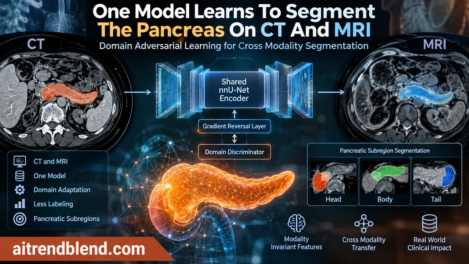
Key Points
- Researchers from Northwestern and Mayo Clinic trained one segmentation model across 4,604 CT and MRI scans using domain adversarial learning to force the encoder to represent pancreatic anatomy rather than scanner specific appearance.
- The unified model reached an average Dice score of 87.31 percent on held out test data and stayed between 84.20 percent and 88.09 percent across four external datasets it never trained on.
- The same encoder was then frozen and reused to segment the pancreatic head, body, and tail, reaching 83.05 percent Dice on CT scans despite never seeing a single CT subregion label during that stage.
- A gradient reversal layer sits at the center of the method, actively punishing the encoder whenever it learns features that reveal which scanner type produced an image.
- The approach is a research framework validated on retrospective data, not an approved clinical tool, and the authors themselves flag several open questions about scanner level variation and other organs.
Not Medical Advice
This article explains a published research preprint. It is not medical advice, a diagnostic tool, or a treatment recommendation. Decisions about pancreatic imaging, cyst monitoring, or cancer screening should be made with a qualified radiologist, gastroenterologist, or oncologist rather than based on anything summarized here.
Why pancreas segmentation splinters across CT and MRI
The pancreas is already one of the harder organs to segment automatically. It sits deep in the abdomen, changes shape substantially from person to person, and offers relatively low contrast against the fat, bowel, and blood vessels surrounding it. Add a second imaging modality into the mix and the difficulty compounds. CT and MRI do not just look different, they measure fundamentally different physical properties, X-ray attenuation for CT versus proton behavior in a magnetic field for MRI, and within MRI itself, different sequences such as T1W, T2W, and the out of phase variant, abbreviated OOP, each render soft tissue with its own distinct intensity pattern.
In a typical hospital, this variety is not an edge case, it is routine. Abdominal imaging protocols mix modalities and sequences depending on the clinical question, the referring physician’s preference, and what equipment happens to be available that day. Training a completely separate segmentation model for every combination is inefficient at best and often simply impossible, since annotated data for some of those combinations, MRI subregion labels in particular, is scarce. The naive fix, pooling all the CT and MRI data together and training one ordinary model on the mixture, tends to backfire. The authors of this new paper describe exactly why. A model trained this way tends to latch onto modality specific appearance cues, essentially learning shortcuts tied to how CT or MRI happens to look, rather than learning what a pancreas actually is anatomically. The result is a model that performs unevenly and unpredictably once it meets a scan type it has not memorized well.
What domain adversarial learning actually forces the model to do
The fix the paper proposes borrows a well known idea from the broader domain adaptation literature, the Domain-Adversarial Neural Network, often shortened to DANN, first introduced in 2016. The core trick is a small architectural addition called a gradient reversal layer, positioned between the model’s encoder and a second, separate network called a domain discriminator.
During the forward pass, the gradient reversal layer does nothing at all, it simply passes the encoder’s features through unchanged to the discriminator, whose only job is to guess whether a given set of features came from a CT scan or an MRI scan. But during backpropagation, the layer flips the sign of the gradient flowing back from that discriminator into the encoder. In practice this means the encoder is being trained to actively confuse the discriminator rather than help it. Every time the discriminator gets better at telling CT features from MRI features, that same signal, reversed, pushes the encoder to erase whatever cue the discriminator just exploited. Play that tug of war out over enough training steps and the encoder is left representing only the anatomical structure that both modalities share, since anything modality specific keeps getting punished out of existence.
That last equation hides a genuinely practical detail. If the adversarial pressure were turned on at full strength from the very first training step, the encoder would likely never learn to segment anything useful in the first place, since it would be fighting two objectives at once before it has learned either. The researchers instead use a warm up schedule, starting lambda at zero and gradually raising it to a maximum of 0.5 as training proceeds, so the model first becomes competent at the underlying segmentation task before the adversarial pressure to forget modality specific cues kicks in.
Building one encoder that works for both scan types
The overall segmentation network is a fairly standard nnU-Net, the self configuring framework that has become something of a default choice across medical image segmentation because it automatically adapts its architecture and preprocessing to whatever dataset it is given. What makes this paper’s setup notable is not the backbone itself but how it gets trained. A shared encoder and decoder process both CT and MRI volumes through the same weights. Latent features coming out of the encoder feed two separate places at once, forward into the decoder for the actual segmentation prediction, and, through the gradient reversal layer, into the domain discriminator for the adversarial signal described above. The decoder itself is trained with an ordinary combination of Dice loss and cross entropy loss, the same pairing used in countless segmentation papers, chosen because Dice rewards overall volumetric overlap while cross entropy rewards getting individual voxels right.
Training happened in two deliberate stages rather than all at once. The first stage ran for 2,000 epochs using only the segmentation loss, letting the network first become genuinely good at finding the pancreas before anything adversarial entered the picture. The second stage then ran for another 1,000 epochs with the domain discriminator active, gradually applying the adversarial pressure through the warm up schedule described earlier. Notably, the domain label the discriminator has to guess is coarse, simply CT versus MRI, rather than trying to separate T1W from T2W from OOP within MRI. The authors justify this with a t-SNE visualization showing that different MRI sequences already cluster close together in feature space on their own, while the real dividing line sits between CT and MRI as a whole, so there was little reason to make the discriminator’s job harder than it needed to be.
Transferring the encoder to segment head, body, and tail, without CT labels
The more clinically interesting half of the paper is what happens after that shared encoder exists. Knowing where the pancreas is overall is useful, but many real applications, including monitoring pancreatic cysts for early signs of cancer, care about which specific part of the organ, the head, the body, or the tail, a finding sits in, since that location can change surgical planning and risk assessment.
Fine grained subregion labels like this are expensive to produce and, in this study, existed only for the MRI portion of the data, from a dataset called Cyst-X. Rather than trying to collect matching CT subregion labels, which the authors note reflects a genuinely common real world constraint rather than a shortcut, they instead froze the domain invariant encoder entirely and trained only a new, separate decoder on top of it using the available MRI subregion labels. The logic is straightforward once you see it. If the encoder has genuinely learned modality invariant anatomical features rather than modality specific shortcuts, then a decoder trained to read pancreatic subregions out of those features using MRI data alone should, in principle, also work reasonably well when fed the same kind of features extracted from a CT scan, even though it never once saw a CT subregion label during its own training.
The data behind the numbers
The scale of the dataset here is worth pausing on, since it is unusually large for this specific organ and task combination. The in distribution collection totals 4,604 scans, split 8 to 1 to 1 into training, validation, and test sets. On the MRI side this includes the Cyst-X dataset and a private MRI collection, and on the CT side it includes AbdomenCT-1K, a large public abdominal organ dataset, and a separate cohort focused on peri pancreatic edema. Only Cyst-X carries the fine grained head, body, and tail labels needed for the subregion task, which is exactly why that downstream stage had to rely on transfer rather than direct training.
To test generalization honestly, the team also evaluated on four external, out of distribution datasets the model never trained on at all, AMOS in both its CT and MRI forms, BTCV, and U-Mamba. Because these external sets lacked the fine grained subregion annotations needed to test the downstream task, an expert radiologist manually segmented the pancreatic head, body, and tail for a subset, seven scans from AMOS and ten from BTCV, specifically to allow a fair test of subregion transfer on genuinely unseen CT data.
The numbers, and what they actually show
| Dataset | Modality | Dice (%) | IoU (%) |
|---|---|---|---|
| In distribution test, overall | Mixed | 87.31 | 78.42 |
| In distribution test, T2W | MRI | 88.27 | 80.06 |
| In distribution test, OOP | MRI | 89.76 | 82.67 |
| In distribution test, CT | CT | 87.53 | 78.33 |
| AMOS, out of distribution | CT | 84.20 | 74.29 |
| AMOS, out of distribution | MRI | 86.87 | 77.79 |
| BTCV, out of distribution | CT | 84.58 | 73.64 |
| U-Mamba, out of distribution | MRI | 88.09 | 79.34 |
Whole pancreas segmentation holds up surprisingly well outside the training distribution
The headline number is an average Dice score of 87.31 percent on the in distribution held out test set, which is a genuinely strong result for pancreas segmentation, an organ notorious for lower scores than, say, the liver or kidneys in most published benchmarks. What stands out more is the out of distribution behavior. Every single external dataset, spanning both CT and MRI and drawn from institutions and scanners the model never saw during training, still scored above 84 percent Dice, with no additional fine tuning performed on any of them. That is a meaningfully different claim than simply performing well on a held out split of the same source cohorts, since out of distribution testing is specifically designed to catch models that quietly memorized scanner or protocol quirks rather than learning transferable anatomy.
Within the MRI sequences, T2W images produced the tightest boundary accuracy, with a 95th percentile Hausdorff distance of 2.923 millimeters, the lowest of any subgroup, suggesting the model traced the organ’s actual edge with unusual precision on that sequence. The OOP sequence produced the single highest Dice and IoU scores overall, at 89.76 percent and 82.67 percent respectively, while CT performance landed in a comparable middle ground at 87.53 percent, evidence that the cross modality alignment strategy genuinely narrowed the usual gap between CT and MRI performance rather than simply favoring whichever modality had more training data.
Subregion segmentation transfers to CT with zero CT subregion labels
This is the result the paper is really built around, and it deserves to be stated plainly. The frozen, modality invariant encoder, paired with a decoder trained exclusively on MRI subregion labels, reached 83.05 percent average Dice when applied to segmenting the pancreatic head, body, and tail on CT scans, a modality it received zero subregion supervision for. For context, that CT subregion score actually edged out the 80.53 percent achieved on MRI itself, the modality the decoder was actually trained on, which is a somewhat counterintuitive outcome the authors do not fully explain but which at minimum indicates the CT result is not simply a degraded echo of the MRI performance.
| Modality | Subregion | Dice (%) | HD95 (mm) |
|---|---|---|---|
| MRI | Head | 85.19 | 3.402 |
| MRI | Body | 80.23 | 5.289 |
| MRI | Tail | 76.18 | 5.944 |
| CT | Head | 82.29 | 4.901 |
| CT | Body | 83.26 | 4.613 |
| CT | Tail | 83.61 | 3.355 |
Looking at the subregion breakdown, the pancreatic head was consistently the easiest structure to find on MRI, reaching 85.19 percent Dice, likely because the head is the largest and most anatomically distinct of the three subregions, sitting close to the duodenum in a fairly consistent position. The tail told the opposite story on MRI, dropping to 76.18 percent, which tracks with what radiologists already know about the pancreatic tail being smaller, more variable in position, and harder to distinguish from the adjacent spleen and stomach. Interestingly, that pattern essentially flipped on CT, where the tail actually scored highest among the three subregions at 83.61 percent. The paper does not dwell on why, but it does note that CT subregion boundaries showed unusually low distance based error overall, an average 95th percentile Hausdorff distance of just 4.290 millimeters, suggesting that whatever anatomical structure the transferred features are keying on translates into stable, well localized boundaries even where raw overlap scores vary.
Less MRI data still benefits from the domain adversarial pretraining
A separate ablation experiment tested what happens with less downstream supervision, fine tuning the subregion decoder on only 10 percent, 50 percent, or 100 percent of the available T1W or T2W training data, then checking performance on both MRI and CT test sets. Across essentially every setting, the version of the model built on the domain adversarial encoder matched or beat an equivalent baseline built without that adversarial pretraining. The gap was largest on the MRI test set after fine tuning on the full T1W dataset, and on the CT test set the advantage showed up most clearly at the smaller 10 percent and 50 percent T2W data points, exactly the low label regime where a more robust starting representation should matter most. A few settings, particularly some T1W and full data T2W combinations on the CT side, showed only marginal differences, which the authors read honestly rather than glossing over, concluding that the benefit of the domain invariant pretraining depends on both which MRI sequence gets used for fine tuning and how much labeled data is available.
Worth Remembering
The subregion decoder never saw a single CT scan paired with a CT subregion label during its own training. Every CT head, body, and tail prediction in this study came from features the encoder learned while looking only at whole organ labels across both modalities plus MRI specific subregion labels, nothing more.
What the feature space visualizations reveal
Beyond the accuracy numbers, the authors include a genuinely illustrative piece of evidence, a t-SNE projection of the bottleneck features the encoder produces, comparing a version trained without the domain discriminator against the full adversarial version. Without adversarial training, CT and MRI features form two cleanly separated clusters in this projection, a direct visual signature of the modality induced domain shift the whole paper is trying to solve. Features from different MRI sequences, by contrast, mostly overlap with each other even in this baseline version, supporting the earlier decision to treat MRI as one unified domain rather than splitting it further. After the domain discriminator gets introduced, that CT versus MRI separation visibly softens, with points from both modalities beginning to intermingle rather than sitting in two distinct islands.
Without domain adversarial training, CT and MRI features form clearly separated clusters, indicating a strong modality induced domain shift. Hong et al., arXiv preprint, 2026
The authors are careful to flag that a t-SNE plot is a qualitative illustration rather than a quantitative proof, points that look close together in a two dimensional projection are not a rigorous measure of anything, but they note it lines up with the harder quantitative evidence, the out of distribution Dice scores and the subregion transfer results, all pointing the same direction.
The clinical translation gap
It is worth being direct about the distance between this result and anything that could influence patient care today. The paper describes a research framework, validated retrospectively against existing annotated datasets, not a deployed or regulatory cleared clinical tool. Every scan used here was already collected and already had, or eventually received, expert ground truth labels. Real world deployment would require prospective validation, meaning testing the model on new patients as they are scanned in ordinary clinical workflow, plus its own regulatory pathway before it could reasonably influence a diagnosis, a surgical plan, or a cyst monitoring decision.
There is also a specific translation question the paper itself raises about scope. The framework aligns CT and MRI as two broad categories, but real clinical imaging varies along other axes too, different scanner manufacturers, different field strengths, different acquisition protocols even within the same modality. The authors explicitly note that their experiments and feature analysis point to modality level shift, CT versus MRI, as the dominant source of the problem they observed, while finer grained factors like scanner or protocol variation were set aside as future work rather than something this study directly measured. Anyone considering this approach for a specific hospital’s imaging fleet should treat that as an open question rather than an assumption.
Honest limitations
The paper is candid about several boundaries on what these results support, and they are worth listing plainly rather than glossing over.
First, the subregion transfer result, while the paper’s most striking finding, was only rigorously validated against expert ground truth for a modest number of external CT scans, seventeen total across the AMOS and BTCV subsets that a radiologist manually annotated specifically for this purpose. That is a meaningful validation step, since it involved genuinely independent expert labeling rather than relying on the model’s own outputs, but seventeen scans is still a small sample for drawing sweeping conclusions about how reliably this transfer would hold across the full diversity of real world CT pancreatic anatomy.
Second, the adversarial training schedule itself, the warm up length, the maximum lambda value of 0.5, the two stage epoch counts, was arrived at empirically to keep training stable in this particular multi stage setup. The authors do not claim these specific values are optimal in any general sense, and different datasets or architectures would likely need their own tuning.
Third, and the authors state this directly, the study centers on a single organ. Nothing here has been tested on other structures, and the paper explicitly leaves extending the framework to other organs as future work rather than a demonstrated capability.
Fourth, the private MRI dataset contributing nearly 1,900 of the 4,604 total scans is, by definition, not independently reviewable by outside readers of this paper, which is common in medical imaging research given patient privacy constraints but still means a meaningful chunk of the training data cannot be scrutinized directly.
Finally, code and trained weights are not yet publicly available. The authors state these will be released upon acceptance, which means independent replication of these exact numbers is not currently possible for outside groups, a normal state of affairs for a fresh preprint but worth knowing if you are trying to build directly on this work today.
Where this goes next
The authors point toward a few specific next steps rather than vague future promises. Extending the domain alignment beyond the coarse CT versus MRI split to account for scanner and protocol level variation is explicitly named as unfinished business, and given how much real world imaging fleets vary even within a single modality, that seems like the most clinically consequential gap to close. Expanding the subregion validation set beyond the current seventeen expert annotated CT scans would also meaningfully strengthen confidence in the downstream transfer claim, since larger, independently reviewed test sets tend to reveal edge cases that smaller ones miss. And the organ specific scope invites an obvious question, whether the same shared encoder plus gradient reversal recipe would transfer as cleanly to other abdominal organs facing similar CT and MRI labeling imbalances, such as the liver or kidneys, where annotated MRI data is also comparatively scarce next to CT.
Conclusion
The core achievement here is a genuinely practical answer to a labeling problem that shows up constantly in medical imaging, not just for the pancreas. Fine grained anatomical annotations are expensive and, in practice, they frequently exist for only one modality at a time, while the other modality sits with only coarse or no labels at all. By forcing a shared encoder to represent anatomy rather than appearance, this framework lets a decoder trained on the well labeled modality do useful work on the poorly labeled one, reaching 83.05 percent Dice on CT pancreatic subregions without a single CT subregion label in sight.
The conceptual shift worth sitting with is subtle but important. This is not a claim that CT and MRI are secretly the same kind of image, they obviously are not. It is a narrower and more defensible claim, that the anatomical structure both modalities are trying to depict can be represented in a shared latent space even when the raw pixel statistics differ enormously, and that an adversarial signal is an effective, relatively lightweight way to push a network toward finding that shared representation rather than shortcutting through modality specific texture.
Transferability beyond the pancreas looks genuinely plausible, even if untested here. Any organ facing a similar pattern, reasonably well labeled in one modality and sparsely labeled in another, liver segments, kidney regions, cardiac chambers imaged across both CT and MRI protocols, could in principle benefit from the same recipe, a shared encoder, a gradient reversal layer, and a frozen transfer step once the upstream representation proves stable.
The honest remaining limitations are real and the authors do not hide them, a validation set of seventeen scans for the headline downstream claim, an empirically tuned rather than theoretically justified training schedule, and a scope that stops at modality level alignment while leaving scanner and protocol level variation for later work. None of that erases the result, but it does mean the appropriate reaction is interest and follow up research rather than immediate clinical adoption.
Where this heads next matters more than where it stands today. If the same approach extends cleanly to finer grained domain shifts, more organs, and larger independently validated test sets, it points toward a genuinely useful pattern for medical imaging AI more broadly, squeezing far more clinical value out of the fine grained labels that already exist in one modality, rather than waiting for someone to painstakingly recreate those same labels in every modality a hospital happens to use.
Reference implementation
The architecture at the center of this paper has three moving parts worth seeing in code, a shared segmentation encoder and decoder, a gradient reversal layer, and a lightweight domain discriminator, trained with the combined loss described above. The implementation below is a simplified, runnable 3D version built for clarity rather than production use, following the paper’s described components and training schedule.
import torch
import torch.nn as nn
import torch.nn.functional as F

# ---------------------------------------------------------------------------
# 1. Gradient Reversal Layer
#    Identity on the forward pass, sign-flipped gradient on the backward pass.
# ---------------------------------------------------------------------------
class GradientReversalFunction(torch.autograd.Function):
    @staticmethod
    def forward(ctx, x, lambd):
        ctx.lambd = lambd
        return x.view_as(x)

    @staticmethod
    def backward(ctx, grad_output):
        return -ctx.lambd * grad_output, None


class GradientReversalLayer(nn.Module):
    def __init__(self):
        super().__init__()

    def forward(self, x, lambd=1.0):
        return GradientReversalFunction.apply(x, lambd)


# ---------------------------------------------------------------------------
# 2. A compact 3D encoder-decoder standing in for the paper's nnU-Net backbone
# ---------------------------------------------------------------------------
class ConvBlock3D(nn.Module):
    def __init__(self, in_ch, out_ch):
        super().__init__()
        self.block = nn.Sequential(
            nn.Conv3d(in_ch, out_ch, kernel_size=3, padding=1),
            nn.InstanceNorm3d(out_ch),
            nn.LeakyReLU(0.01, inplace=True),
            nn.Conv3d(out_ch, out_ch, kernel_size=3, padding=1),
            nn.InstanceNorm3d(out_ch),
            nn.LeakyReLU(0.01, inplace=True),
        )

    def forward(self, x):
        return self.block(x)


class PancreasEncoder(nn.Module):
    def __init__(self, in_channels=1, base_ch=16):
        super().__init__()
        self.enc1 = ConvBlock3D(in_channels, base_ch)
        self.enc2 = ConvBlock3D(base_ch, base_ch * 2)
        self.enc3 = ConvBlock3D(base_ch * 2, base_ch * 4)
        self.bottleneck = ConvBlock3D(base_ch * 4, base_ch * 8)
        self.pool = nn.MaxPool3d(2)

    def forward(self, x):
        s1 = self.enc1(x)
        s2 = self.enc2(self.pool(s1))
        s3 = self.enc3(self.pool(s2))
        z = self.bottleneck(self.pool(s3))
        return z, (s1, s2, s3)


class PancreasDecoder(nn.Module):
    # A task-specific decoder. Used both for whole pancreas segmentation
    # and, in a second frozen-encoder instance, for subregion segmentation.
    def __init__(self, base_ch=16, out_channels=1):
        super().__init__()
        self.up3 = nn.ConvTranspose3d(base_ch * 8, base_ch * 4, kernel_size=2, stride=2)
        self.dec3 = ConvBlock3D(base_ch * 8, base_ch * 4)
        self.up2 = nn.ConvTranspose3d(base_ch * 4, base_ch * 2, kernel_size=2, stride=2)
        self.dec2 = ConvBlock3D(base_ch * 4, base_ch * 2)
        self.up1 = nn.ConvTranspose3d(base_ch * 2, base_ch, kernel_size=2, stride=2)
        self.dec1 = ConvBlock3D(base_ch * 2, base_ch)
        self.out_conv = nn.Conv3d(base_ch, out_channels, kernel_size=1)

    def forward(self, z, skips):
        s1, s2, s3 = skips
        d3 = self.dec3(torch.cat([self.up3(z), s3], dim=1))
        d2 = self.dec2(torch.cat([self.up2(d3), s2], dim=1))
        d1 = self.dec1(torch.cat([self.up1(d2), s1], dim=1))
        return self.out_conv(d1)


class DomainDiscriminator(nn.Module):
    # Predicts CT (1) vs MRI (0) from pooled bottleneck features.
    def __init__(self, in_ch=128):
        super().__init__()
        self.pool = nn.AdaptiveAvgPool3d(1)
        self.classifier = nn.Sequential(
            nn.Linear(in_ch, 64),
            nn.ReLU(inplace=True),
            nn.Linear(64, 2),
        )

    def forward(self, z):
        pooled = self.pool(z).flatten(1)
        return self.classifier(pooled)


# ---------------------------------------------------------------------------
# 3. Loss functions
# ---------------------------------------------------------------------------
def dice_loss(pred_logits, target, eps=1e-6):
    pred = torch.sigmoid(pred_logits)
    dims = (2, 3, 4)
    intersection = (pred * target).sum(dim=dims)
    union = pred.sum(dim=dims) + target.sum(dim=dims)
    dice = (2 * intersection + eps) / (union + eps)
    return 1 - dice.mean()


def segmentation_loss(pred_logits, target):
    return dice_loss(pred_logits, target) + F.binary_cross_entropy_with_logits(pred_logits, target)


# ---------------------------------------------------------------------------
# 4. Full model wiring encoder, decoder, GRL, and discriminator together
# ---------------------------------------------------------------------------
class UnifiedPancreasModel(nn.Module):
    def __init__(self, base_ch=16):
        super().__init__()
        self.encoder = PancreasEncoder(in_channels=1, base_ch=base_ch)
        self.decoder = PancreasDecoder(base_ch=base_ch, out_channels=1)
        self.grl = GradientReversalLayer()
        self.discriminator = DomainDiscriminator(in_ch=base_ch * 8)

    def forward(self, x, lambd=0.0):
        z, skips = self.encoder(x)
        seg_logits = self.decoder(z, skips)
        domain_logits = self.discriminator(self.grl(z, lambd))
        return seg_logits, domain_logits


# ---------------------------------------------------------------------------
# 5. Training loop skeleton with the warm-up lambda schedule from the paper
# ---------------------------------------------------------------------------
def lambda_schedule(epoch, warmup_epochs=2000, adv_epochs=1000, lambda_max=0.5):
    if epoch < warmup_epochs:
        return 0.0
    progress = min(1.0, (epoch - warmup_epochs) / max(1, adv_epochs))
    return lambda_max * progress


def train_step(model, optimizer, images, masks, domain_labels, epoch):
    model.train()
    optimizer.zero_grad()

    lambd = lambda_schedule(epoch)
    seg_logits, domain_logits = model(images, lambd=lambd)

    seg = segmentation_loss(seg_logits, masks)
    dom = F.cross_entropy(domain_logits, domain_labels)
    total = (1 - lambd) * seg + lambd * dom

    total.backward()
    optimizer.step()
    return {"seg_loss": seg.item(), "domain_loss": dom.item(), "total_loss": total.item()}


# ---------------------------------------------------------------------------
# 6. Dice evaluation on binarized predictions
# ---------------------------------------------------------------------------
@torch.no_grad()
def evaluate_dice(model, images, masks, threshold=0.5):
    model.eval()
    seg_logits, _ = model(images, lambd=0.0)
    pred = (torch.sigmoid(seg_logits) > threshold).float()
    dims = (2, 3, 4)
    intersection = (pred * masks).sum(dim=dims)
    union = pred.sum(dim=dims) + masks.sum(dim=dims)
    dice = (2 * intersection + 1e-6) / (union + 1e-6)
    return dice.mean().item()


# ---------------------------------------------------------------------------
# 7. Smoke test on dummy data, confirms the full pipeline runs end to end
# ---------------------------------------------------------------------------
if __name__ == "__main__":
    torch.manual_seed(0)

    batch_size, depth, height, width = 2, 32, 64, 64
    dummy_images = torch.randn(batch_size, 1, depth, height, width)
    dummy_masks = (torch.rand(batch_size, 1, depth, height, width) > 0.7).float()
    dummy_domain_labels = torch.tensor([1, 0])  # one CT scan, one MRI scan

    model = UnifiedPancreasModel(base_ch=8)
    optimizer = torch.optim.Adam(model.parameters(), lr=1e-3)

    print("Running warm-up stage smoke test, lambda should be 0")
    stats = train_step(model, optimizer, dummy_images, dummy_masks, dummy_domain_labels, epoch=100)
    print(stats)

    print("Running adversarial stage smoke test, lambda should be greater than 0")
    stats = train_step(model, optimizer, dummy_images, dummy_masks, dummy_domain_labels, epoch=2500)
    print(stats)

    dice = evaluate_dice(model, dummy_images, dummy_masks)
    print(f"Dummy Dice score after two training steps: {dice:.4f}")
This reference version simplifies several things the real paper handles more carefully, most notably the full nnU-Net preprocessing pipeline, its automatic architecture configuration, and the sliding window inference used to stitch predictions back into full volumes. It keeps the three components that actually define this method, the gradient reversal layer, the shared encoder feeding both a segmentation decoder and a domain discriminator, and the warm up schedule that keeps the adversarial signal from overwhelming training before the model has learned to segment anything at all.
Frequently Asked Questions
What problem does domain adversarial learning solve in this pancreas segmentation paper
It solves the problem of a single model performing unevenly across CT and MRI scans because it learns to rely on modality specific appearance cues instead of stable anatomical structure. A gradient reversal layer actively penalizes the encoder whenever its features reveal which scanner type produced an image, pushing it toward representations that generalize across both modalities.
How accurate was the unified model at segmenting the whole pancreas
The model reached an average Dice score of 87.31 percent on the in distribution test set, and stayed between 84.20 percent and 88.09 percent across four separate external datasets it never trained on, spanning both CT and MRI.
How can the model segment CT subregions without ever seeing CT subregion labels
The encoder is trained first to be modality invariant across CT and MRI using whole pancreas labels from both. It is then frozen, and a new decoder is trained only on MRI subregion labels. Because the frozen features already represent anatomy rather than modality specific appearance, that same decoder can be applied directly to CT scans and still localize the head, body, and tail reasonably well.
What Dice score did the model achieve for pancreatic head, body, and tail segmentation
It reached 80.53 percent average Dice on MRI, the modality it was actually fine tuned on, and 83.05 percent average Dice on CT despite receiving no CT subregion supervision during that stage.
Is this pancreas segmentation model ready to use in a hospital
No. It is a research framework validated on retrospective data with code and trained weights not yet publicly released. The authors describe it as a demonstration that unified anatomical representations can work across modalities, not as an approved or deployed clinical tool, and they flag several open questions about scanner and protocol level variation that remain untested.
Could this same approach work for organs other than the pancreas
The authors state that extending the framework to other organs remains future work and was not tested in this study. In principle, any organ with well labeled data in one modality and sparse labels in another, such as certain liver or kidney segmentation tasks, could be a reasonable candidate for the same shared encoder and gradient reversal approach.
Read the full preprint for the complete architecture details, the t-SNE feature analysis, and the ablation results.
This analysis is based on the published preprint and an independent evaluation of its claims.