
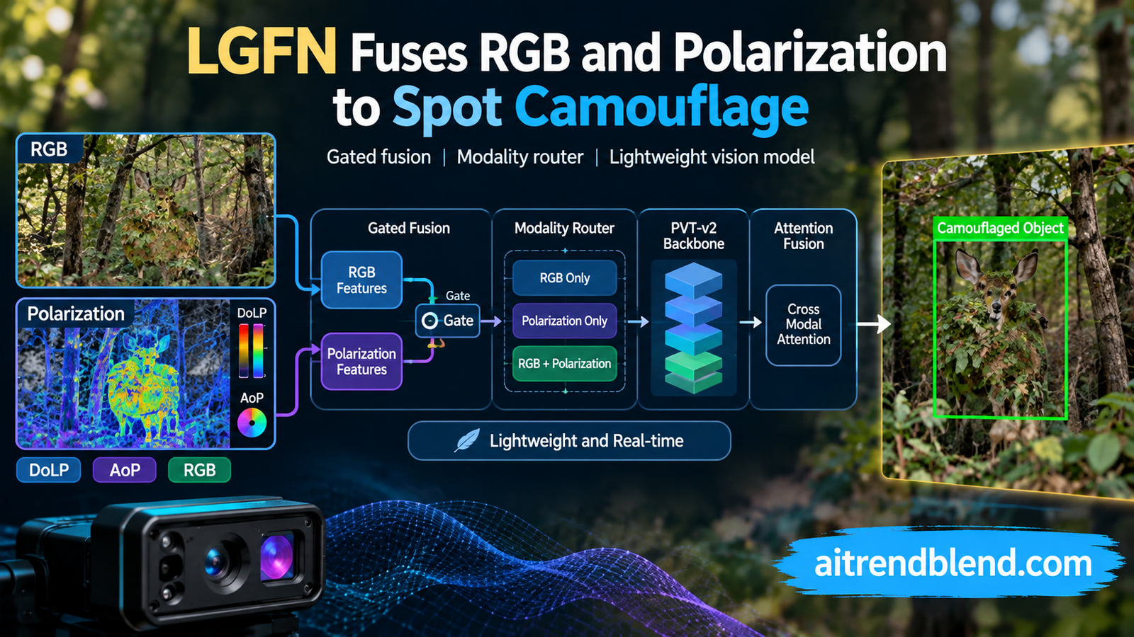
Point a camera at a stick insect on a branch and your eye does most of the work without you noticing. A neural network does not have that luxury. When a target shares the same color and texture as everything behind it, the pixels alone stop carrying enough evidence, and even strong segmentation models start guessing. A team from Foshan University and China University of Mining and Technology in Beijing decided the missing evidence was physical, not visual, and they built a model around a light property that human eyes ignore.
Key points
- LGFN adds polarization cues, the degree of linear polarization and the angle of polarization, to ordinary RGB so it can separate objects that look identical to the background.
- A deterministic Modality Router picks an RGB only path or a multimodal path based purely on which sensors are present, with no learned quality score at inference.
- The design keeps polarization coordination separate from RGB interaction, so the two do not fight inside one overloaded module.
- On the 230 image PCOD_1200 test set the RGB only route reaches a mean absolute error of 0.0090 and an intersection over union of 0.8144, the top score on all six metrics reported.
- The RGB only route runs in about 7.40 ms per image with 25.10 M parameters, and the multimodal route cuts parameters, compute, and latency well below the previous polarization method IPNet.
- A complete and runnable PyTorch reference implementation is included at the end of this article.
Why RGB alone runs out of clues
Camouflaged object detection, usually shortened to COD, asks a model to segment things that evolved or were designed to disappear. Concealed animals, hidden defects, objects under military or industrial cover. The whole difficulty is that the target does everything it can to look like its surroundings, which means weak edges, broken outlines, and foreground regions whose brightness and hue match the background almost perfectly.
Most modern COD systems attack this with cleverer use of the same RGB pixels. They add contextual reasoning, multiple scales, structural priors, boundary attention, and the kind of transformer style feedback we track across the vision and attention pillar. These methods have pushed the field a long way. The problem runs deeper than better feature mixing can fix. Every one of those signals still comes from appearance, and appearance is exactly what a camouflaged object corrupts on purpose. When the surface reflectance and the local geometry of a target are visually close to the scene, no amount of RGB reasoning invents information that the sensor never captured.
Polarization is where that extra information lives. Light bouncing off a surface picks up a polarization signature that depends on the material, its roughness, and the angle of the surface relative to the camera. Two regions can look the same shade of brown to a normal camera while carrying very different polarization responses, because one is a leaf and the other is a beetle. Researchers describe this with two quantities. The degree of linear polarization, written DoLP, measures how strongly the reflected light is polarized. The angle of polarization, written AoP, describes the dominant orientation of that polarization. Together they expose target and background differences that stay invisible in ordinary color.
The core idea. RGB tells you what a surface looks like. Polarization tells you something about what the surface is and how it sits in space. For a camouflaged object, the second question is often the only one with a useful answer.
The gap the authors actually target
Polarization assisted COD is not brand new. PolarNet showed the idea was feasible, and IPNet introduced the PCOD_1200 benchmark with a dual flow RGB and polarization network. So why write another paper? Because the earlier systems made two assumptions that break in practice.
First, they treated polarization as more appearance channels and pushed DoLP, AoP, and RGB into a single tightly coupled fusion module. That forces one block to resolve two very different problems at once. DoLP and AoP disagree with each other in their own ways, an issue the authors call intra polarization heterogeneity, and both disagree with the RGB representation. Cramming all of that into one interaction step tends to let uncoordinated polarization noise leak into the RGB features that were doing most of the honest work.
Second, earlier methods assumed the polarization inputs are always there. Real sensing rigs are messier. A DoLP channel might be available while AoP is not, or a deployment might have only an ordinary RGB camera. A model that hardwires polarization into its forward pass either wastes computation running dead branches or simply cannot run at all when a modality is missing.
LGFN, short for Lightweight Gated RGB Polarization Fusion, is built to answer both problems. It coordinates the polarization cues among themselves before it ever lets them touch the RGB stream, and it adapts its own computation to whatever sensors happen to be present. The name to keep in mind is that RGB stays the principal pathway throughout. Polarization is a guest that gets invited in carefully, not a co host that rearranges the furniture.
A router that refuses to guess
The first design decision is the one most papers overcomplicate. How should a model decide when to use polarization? A tempting answer is to learn a quality estimator that scores each input and blends predictions. LGFN goes the other way. It uses a deterministic Modality Router that looks only at availability.
The authors define a modality availability vector where RGB is always mandatory and two binary flags mark whether DoLP and AoP are present. If neither polarization input exists, the router sends the image down a dedicated RGB only route that behaves like a conventional segmentation pipeline. If at least one polarization input exists, the router activates the multimodal route.
What matters here is what the router does not do. It never estimates sample specific input quality and it never combines predictions from multiple routes. That sounds almost too simple, and that is the point. A learned quality gate is one more thing that can be wrong, and when it is wrong on a hard camouflaged scene it fails exactly when you need it most. A rule based on which physical sensor is connected cannot hallucinate. The two routes are also trained and stored as separate checkpoints, each optimized for its own job, so the RGB only deployment carries none of the multimodal overhead.
Three stages that each do one thing
Everything interesting happens inside the multimodal route, and its cleanest feature is discipline. Instead of one giant fusion block, the work is split across three stages that run in order. A Modality Gate decides how much say each polarization branch gets. A Gated Polarization Hub coordinates the polarization evidence with itself. An RGB Polarization Cross Fusion step finally injects that coordinated evidence into the RGB hierarchy. Read that sequence again, because the ordering is the whole argument of the paper.
Stage one, the Modality Gate
The RGB image runs through a PVT-v2-B2 backbone, while DoLP and AoP each get their own lightweight encoder with separate weights. Before any of those features interact, a small multilayer perceptron reads the availability vector and produces three numbers. Two control how much weight DoLP and AoP each receive, and the third controls the overall strength of polarization injection.
The weights come from a masked softmax that zeroes out any branch whose sensor is absent and normalizes the survivors so they sum to one.
A separate bounded coefficient governs the global injection strength, kept inside a safe range so polarization can be dialed down but never allowed to dominate.
Notice what the gate is allowed to see, which is only the availability vector. It never looks at image content, handcrafted statistics, or sample level quality descriptors. So the gate is deciding allocation policy, not judging individual pictures. That is a deliberately humble module, and the ablations later show the humility pays off.
Stage two, the Gated Polarization Hub
Now the polarization cues get organized among themselves. The Gated Polarization Hub, called GPH, combines the weighted DoLP and AoP features with a set of explicit polarization cues at four scales.
Those explicit cues are worth a moment. Hierarchical encoders are good at semantics but tend to smooth away fine boundaries and contrast, which are precisely the thin signals that betray a camouflaged edge. So the authors build an eight channel cue tensor straight from the raw maps. It carries the masked DoLP and AoP maps, their first order gradient magnitudes, their 5×5 local residuals, and the maximum gradient and residual responses across whichever polarization modalities are available. A small encoder turns that into scale aligned structure that the learned features can lean on. It is a nice reminder that not every useful feature has to be learned from scratch.
The aggregated representation then passes through a scale specific convolution with batch normalization and a rectified linear unit, followed by a squeeze and excitation style channel recalibration that emphasizes informative polarization responses and suppresses redundant ones.
By the time GPH finishes, the heterogeneous polarization evidence has been reconciled into one coordinated representation per scale. Crucially it has done this inside the polarization domain, without dragging RGB into the argument. The RGB features are still clean.
Stage three, RGB Polarization Cross Fusion
Only now does polarization meet RGB. The RGB Polarization Cross Fusion module, called RPCF, is intentionally asymmetric. It treats the coordinated polarization feature as a correction to add to RGB, not as an equal partner to average with it. At each scale, the RGB feature and the coordinated polarization feature are concatenated and projected into a residual candidate.
The residual candidate is sharpened by parallel spatial and channel attention, then added back to the original RGB feature through an identity shortcut. The residual scale is fixed at 1.5 across all experiments, and the injection coefficient from the gate multiplies it. Because of the identity shortcut, when no polarization is available the injection coefficient falls to zero and the whole module collapses back to plain RGB. That case is only a mathematical fallback though, since the router already sends sensor free inputs to the dedicated RGB only route.
The four fused representations feed a feature pyramid style decoder that produces the final camouflage probability map. Take a step back and the flow is easy to state. Weight the polarization branches by availability, coordinate them in their own domain, then inject the result into RGB as a controlled residual that can never overwhelm the main signal.
How it is trained
The loss design mirrors the architecture. A structure aware segmentation objective combines weighted binary cross entropy, weighted intersection over union, and Dice loss, with a weight map that emphasizes structurally ambiguous boundary regions. Edge supervision comes from the morphological difference between dilated and eroded ground truth masks, which is a tidy way to manufacture an edge target without extra labeling.
Two auxiliary multimodal objectives run only during training and add no inference cost. A fusion consistency loss keeps a reconstructed fusion map anchored to grayscale RGB appearance while retaining the strongest available structural gradients from DoLP and AoP. A gate loss pushes the learned polarization allocation and injection strength toward fixed offline targets built from training modalities. The full objective ties them together.
The RGB and edge predictions act as training only regularizers weighted at 0.2 and 0.5, while the fusion and gate objectives enter at 0.3 each. All of them disappear at inference, which is how a model this careful still runs fast.
What the numbers actually say
The experiments cover three benchmarks. PCOD_1200, which carries the polarization data, plus fixed subsets of COD10K and NC4K for extra RGB comparison. All inputs are resized to 352 by 352 and the RGB encoder is PVT-v2-B2. The RGB only and multimodal routes are trained and evaluated separately, exactly as they would be deployed.
On the full 230 image PCOD_1200 test set, compared against nine RGB based COD methods, the RGB only route of LGFN takes the top result on every metric reported.
| Method | MAE | Sa | Eφ | Fβw | Dice | IoU |
|---|---|---|---|---|---|---|
| GBNet (2026) | 0.0158 | 0.8840 | 0.9246 | 0.8152 | 0.8249 | 0.7651 |
| DepthSAM (2026) | 0.0140 | 0.8870 | 0.9213 | 0.8149 | 0.8245 | 0.7714 |
| LGFN (RGB only) | 0.0090 | 0.9162 | 0.9637 | 0.8688 | 0.8806 | 0.8144 |
Cutting mean absolute error from the next best 0.0140 down to 0.0090 is a real gap, not a rounding win, and the intersection over union climbs from 0.7714 to 0.8144 at the same time. The qualitative figures back this up. LGFN produces more complete masks and suppresses distracting background responses in scenes with weak contrast and fragmented structure.
On the RGB only subsets the story is more honest and more believable for it. On the 405 image COD10K subset, LGFN ranks around third across most metrics rather than first, and the authors say so plainly. On the 200 image NC4K subset it wins the enhanced alignment measure at 0.9874 and the Dice score, while sitting second on several others. A model that claimed to win everything everywhere would be more suspicious than one that wins its home benchmark decisively and stays competitive elsewhere.
The polarization assisted comparison is where the full design earns its keep. Against PolarNet and IPNet on the complete PCOD_1200 test set, the multimodal route leads on all six metrics.
| Method | MAE | Sa | Eφ | Fβw | Dice | IoU |
|---|---|---|---|---|---|---|
| PolarNet (2023) | 0.0473 | 0.6610 | 0.7718 | 0.4537 | 0.4392 | 0.3403 |
| IPNet (2024) | 0.0147 | 0.8696 | 0.9342 | 0.8184 | 0.8063 | 0.7162 |
| LGFN (multimodal) | 0.0097 | 0.9045 | 0.9651 | 0.8693 | 0.8678 | 0.7944 |
The region overlap improvement is the one to watch. Dice rises from 0.8063 to 0.8678 and intersection over union from 0.7162 to 0.7944 against IPNet. For camouflaged targets, where the whole game is recovering a complete and correctly bounded region, that is the metric that reflects a genuinely better mask rather than a slightly luckier threshold.
Key takeaway. The multimodal route does not just edge past IPNet, it does so while being far cheaper. Reported gains of roughly five points in region overlap arrive alongside large cuts in parameters and latency, which is an unusual combination.
Lightweight is not a slogan here
Plenty of papers put lightweight in the title and then report a model that is only light on a good day. LGFN backs the claim with numbers. The RGB only route uses 25.10 M parameters and 10.36 G floating point operations, running at about 7.40 ms per image on an A800 GPU at the 352 by 352 resolution. That is the fastest measured latency among the compared models and second smallest in both size and compute.
There is a useful lesson buried in the efficiency table. DGNet has fewer parameters and lower reported floating point operations, yet its measured latency is higher. Theoretical operation counts do not always translate into wall clock speed, because how an operator is implemented and profiled matters as much as how many multiplies it nominally performs. The authors report both estimated compute and real timing rather than hiding behind one number, which is the right way to talk about efficiency.
The multimodal route is heavier at 59.20 M parameters, 24.29 G floating point operations, and 18.46 ms, which is expected since it runs extra encoders. Set against IPNet it still cuts parameter count by 53.1 percent, floating point operations by 73.6 percent, and latency by 63.0 percent, while beating it on every accuracy metric. PolarNet is lighter and faster than the multimodal route, but its segmentation quality is far behind, so the comparison there is not really close.
Do the pieces earn their place?
The ablations are refreshingly direct. Strip out all the proposed components and the model degrades on every metric, with mean absolute error rising from 0.0090 to 0.0112 and intersection over union falling from 0.7944 to 0.7805 under the multimodal protocol.
| Variant | MAE | Sa | Eφ | Fβw | Dice | IoU |
|---|---|---|---|---|---|---|
| Full LGFN | 0.0097 | 0.9045 | 0.9651 | 0.8693 | 0.8678 | 0.7944 |
| Baseline, no modules | 0.0112 | 0.8975 | 0.9602 | 0.8579 | 0.8559 | 0.7805 |
| Without GPH | 0.0111 | 0.8987 | 0.9573 | 0.8557 | 0.8585 | 0.7811 |
| Without RPCF | 0.0098 | 0.9009 | 0.9622 | 0.8589 | 0.8575 | 0.7857 |
| Without Gate | 0.0101 | 0.9016 | 0.9621 | 0.8656 | 0.8626 | 0.7891 |
| Without explicit cues | 0.0107 | 0.9003 | 0.9581 | 0.8585 | 0.8580 | 0.7837 |
Removing the Gated Polarization Hub causes the largest single drop, which lines up with the paper’s central claim that coordinating polarization before cross modal interaction is what really matters. The Modality Gate produces the smallest change on its own, and that is not a weakness. A gate whose job is to allocate policy from availability alone should not be doing heavy lifting on any one image. Its value shows up across the distribution of sensor conditions, not on a single test number. The training objective ablations tell a similar story. Dropping the fusion loss reduces the weighted F measure, Dice, and intersection over union by 0.0173, 0.0223, and 0.0202, so the auxiliary supervision is pulling real weight even though it costs nothing at inference.
Where it still struggles
The authors are candid about limits, and the qualitative failure cases make the honesty concrete. When background polarization is strong, or when target and polarization cues are spatially inconsistent, the multimodal route can add false negatives or false positives rather than removing them. Polarization is complementary evidence, not a guarantee, and a scene that confuses the polarization sensor can drag the fusion down instead of lifting it.
Two structural caveats deserve emphasis for anyone thinking of building on this. The study rests on a single polarization benchmark, PCOD_1200, since polarization COD data is scarce, so the multimodal claims have not been stress tested across many independent datasets the way RGB COD has. And the two routes are trained as separate checkpoints, which is clean for deployment but means the model does not yet share parameters or learn a unified representation across sensor conditions. The authors flag shared parameterization and finer sample level and region level polarization reliability modeling as future work, and both feel like the right next steps rather than afterthoughts.
None of this comes for free either. Polarization imaging needs specialized capture hardware, so the multimodal route is only relevant where a polarization camera actually exists. The RGB only route is the part most readers can use today, and it is strong enough to stand on its own.
Why the design travels
Strip away the polarization specifics and LGFN is a template for adding any auxiliary modality to a model whose main input you trust. The pattern is worth remembering. Decide participation from availability rather than a fragile learned quality score. Reconcile the new modality with itself before it argues with the primary stream. Inject it as a bounded residual so it can help but never take over. Keep the auxiliary supervision in training and out of inference.
That recipe would transfer cleanly to depth sensors, thermal imaging, or event cameras layered onto an RGB detector. The same asymmetry drives work like feature space diffusion for infrared visible fusion and state space models for multimodal fusion, and it fits plenty of settings where a secondary signal is sometimes present and sometimes not. The camouflaged object detection results are the demonstration. The reusable idea is the asymmetric, availability aware fusion discipline underneath them.
Reference implementation in PyTorch
The code below is a faithful and runnable reconstruction of the LGFN multimodal route based on the equations in the paper. It uses a stand in convolutional backbone in place of PVT-v2-B2 so the file runs without external weights, and it includes the Modality Router, the Modality Gate with masked softmax and bounded injection, the Gated Polarization Hub with explicit cues and squeeze and excitation recalibration, the RGB Polarization Cross Fusion residual, an FPN style decoder, the structure aware and auxiliary losses, a training step, an evaluation helper, and a smoke test on dummy tensors. Swap in the real backbone and dataset for actual experiments.
# lgfn_reference.py
# Faithful, runnable reconstruction of the LGFN multimodal route.
# Replace SimpleBackbone with PVT-v2-B2 for real experiments.

import torch
import torch.nn as nn
import torch.nn.functional as F


class SimpleBackbone(nn.Module):
    """Stand in for PVT-v2-B2. Emits four scale features."""
    def __init__(self, in_ch=3, dims=(64, 128, 320, 512)):
        super().__init__()
        self.stem = nn.Conv2d(in_ch, dims[0], 3, 2, 1)
        self.stages = nn.ModuleList()
        prev = dims[0]
        for d in dims:
            self.stages.append(nn.Sequential(
                nn.Conv2d(prev, d, 3, 2, 1),
                nn.BatchNorm2d(d), nn.ReLU(inplace=True),
                nn.Conv2d(d, d, 3, 1, 1),
                nn.BatchNorm2d(d), nn.ReLU(inplace=True)))
            prev = d
        self.dims = dims

    def forward(self, x):
        x = self.stem(x)
        feats = []
        for s in self.stages:
            x = s(x)
            feats.append(x)
        return feats  # list of 4 features, coarse to fine channels


class ModalityGate(nn.Module):
    """Reads only the availability vector m = [1, m_D, m_A]."""
    def __init__(self):
        super().__init__()
        self.mlp = nn.Sequential(
            nn.Linear(3, 16), nn.ReLU(inplace=True),
            nn.Linear(16, 3))  # logits z_D, z_A, z_gamma

    def forward(self, m):
        z = self.mlp(m)                      # (B, 3)
        z_d, z_a, z_g = z[:, 0], z[:, 1], z[:, 2]
        m_d, m_a = m[:, 1], m[:, 2]
        eta = (m_d + m_a > 0).float()      # polarization present flag
        # masked softmax over the two polarization branches
        ed = m_d * torch.exp(z_d)
        ea = m_a * torch.exp(z_a)
        denom = ed + ea + 1e-8
        w_d, w_a = ed / denom, ea / denom
        gamma = eta * (0.3 + 0.7 * torch.sigmoid(z_g))
        return w_d, w_a, gamma, eta


class ExplicitCueEncoder(nn.Module):
    """Builds the 8 channel cue tensor, then encodes to 4 scales."""
    def __init__(self, dims=(64, 128, 320, 512)):
        super().__init__()
        self.enc = SimpleBackbone(in_ch=8, dims=dims)

    def _grad_mag(self, x):
        gx = x[:, :, :, 1:] - x[:, :, :, :-1]
        gy = x[:, :, 1:, :] - x[:, :, :-1, :]
        gx = F.pad(gx, (0, 1, 0, 0))
        gy = F.pad(gy, (0, 0, 0, 1))
        return torch.sqrt(gx ** 2 + gy ** 2 + 1e-6)

    def forward(self, dolp, aop, m_d, m_a):
        b = dolp.shape[0]
        md = m_d.view(b, 1, 1, 1)
        ma = m_a.view(b, 1, 1, 1)
        d, a = dolp * md, aop * ma
        gd, ga = self._grad_mag(d), self._grad_mag(a)
        rd = d - F.avg_pool2d(d, 5, 1, 2)   # 5x5 local residual
        ra = a - F.avg_pool2d(a, 5, 1, 2)
        g_max = torch.max(gd, ga)
        r_max = torch.max(rd.abs(), ra.abs())
        cue = torch.cat([d, a, gd, ga, rd, ra, g_max, r_max], dim=1)
        return self.enc(cue)


class SERecalib(nn.Module):
    def __init__(self, ch, r=8):
        super().__init__()
        self.fc1 = nn.Conv2d(ch, ch // r, 1)
        self.fc2 = nn.Conv2d(ch // r, ch, 1)

    def forward(self, x):
        s = F.adaptive_avg_pool2d(x, 1)
        s = torch.sigmoid(self.fc2(F.relu(self.fc1(s))))
        return x * s


class GPH(nn.Module):
    """Gated Polarization Hub at one scale."""
    def __init__(self, ch):
        super().__init__()
        self.proj = nn.Sequential(
            nn.Conv2d(ch, ch, 3, 1, 1),
            nn.BatchNorm2d(ch), nn.ReLU(inplace=True))
        self.se = SERecalib(ch)

    def forward(self, d_i, a_i, c_i, w_d, w_a, eta):
        b = d_i.shape[0]
        wd = w_d.view(b, 1, 1, 1)
        wa = w_a.view(b, 1, 1, 1)
        u = wd * d_i + wa * a_i + c_i         # Eq 5
        v = self.proj(u)                      # Eq 6
        p = self.se(v)                        # Eq 7
        return p * eta.view(b, 1, 1, 1)


class RPCF(nn.Module):
    """RGB Polarization Cross Fusion, asymmetric residual."""
    def __init__(self, ch):
        super().__init__()
        self.phi = nn.Conv2d(2 * ch, ch, 1)
        self.spatial = nn.Conv2d(ch, 1, 7, 1, 3)
        self.chan = SERecalib(ch)
        self.scale = 1.5                       # fixed residual scale

    def forward(self, r_i, p_i, gamma):
        b = r_i.shape[0]
        delta = self.phi(torch.cat([r_i, p_i], dim=1))   # Eq 8
        s = torch.sigmoid(self.spatial(delta))
        delta_hat = s * self.chan(delta) * delta          # Eq 9
        g = gamma.view(b, 1, 1, 1)
        return r_i + self.scale * g * delta_hat            # identity shortcut


class FPNDecoder(nn.Module):
    def __init__(self, dims, mid=128):
        super().__init__()
        self.lat = nn.ModuleList([nn.Conv2d(d, mid, 1) for d in dims])
        self.head = nn.Conv2d(mid, 1, 1)

    def forward(self, feats):
        x = self.lat[-1](feats[-1])
        for i in range(len(feats) - 2, -1, -1):
            x = F.interpolate(x, size=feats[i].shape[-2:],
                              mode="bilinear", align_corners=False)
            x = x + self.lat[i](feats[i])
        return self.head(x)


class LGFN(nn.Module):
    def __init__(self, dims=(64, 128, 320, 512)):
        super().__init__()
        self.rgb = SimpleBackbone(3, dims)
        self.enc_d = SimpleBackbone(1, dims)
        self.enc_a = SimpleBackbone(1, dims)
        self.cues = ExplicitCueEncoder(dims)
        self.gate = ModalityGate()
        self.gph = nn.ModuleList([GPH(d) for d in dims])
        self.rpcf = nn.ModuleList([RPCF(d) for d in dims])
        self.dec = FPNDecoder(dims)
        self.dec_rgb = FPNDecoder(dims)          # auxiliary RGB head

    def forward(self, rgb, dolp, aop, m):
        r = self.rgb(rgb)
        w_d, w_a, gamma, eta = self.gate(m)
        multimodal = bool((eta > 0).any())
        if not multimodal:                       # deterministic router
            out = self.dec(r)
            return torch.sigmoid(
                F.interpolate(out, size=rgb.shape[-2:],
                              mode="bilinear", align_corners=False)), None
        d, a = self.enc_d(dolp), self.enc_a(aop)
        c = self.cues(dolp, aop, m[:, 1], m[:, 2])
        fused = []
        for i in range(4):
            p = self.gph[i](d[i], a[i], c[i], w_d, w_a, eta)
            fused.append(self.rpcf[i](r[i], p, gamma))
        out = self.dec(fused)
        aux = self.dec_rgb(r)
        up = lambda t: F.interpolate(t, size=rgb.shape[-2:],
                                     mode="bilinear", align_corners=False)
        return torch.sigmoid(up(out)), torch.sigmoid(up(aux))


def structure_loss(pred, mask):
    """Weighted BCE plus weighted IoU, boundary emphasized."""
    w = 1 + 5 * torch.abs(F.avg_pool2d(mask, 31, 1, 15) - mask)
    bce = F.binary_cross_entropy(pred, mask, reduction="none")
    wbce = (w * bce).sum((2, 3)) / w.sum((2, 3))
    inter = ((pred * mask) * w).sum((2, 3))
    union = ((pred + mask) * w).sum((2, 3))
    wiou = 1 - (inter + 1) / (union - inter + 1)
    dice = 1 - (2 * (pred * mask).sum((2, 3)) + 1) / \
        ((pred + mask).sum((2, 3)) + 1)
    return (wbce + wiou + dice).mean()


def train_step(model, opt, batch):
    model.train()
    rgb, dolp, aop, m, gt = batch
    pred, aux = model(rgb, dolp, aop, m)
    loss = structure_loss(pred, gt)
    if aux is not None:
        loss = loss + 0.2 * structure_loss(aux, gt)   # Eq 14 term
    opt.zero_grad()
    loss.backward()
    opt.step()
    return loss.item()


@torch.no_grad()
def evaluate(model, batch):
    model.eval()
    rgb, dolp, aop, m, gt = batch
    pred, _ = model(rgb, dolp, aop, m)
    mae = (pred - gt).abs().mean().item()
    inter = (pred * gt).sum()
    iou = (inter / (pred + gt - pred * gt).sum().clamp(min=1e-6)).item()
    return {"MAE": mae, "IoU": iou}


if __name__ == "__main__":
    # smoke test on dummy data, both routes
    model = LGFN()
    opt = torch.optim.AdamW(model.parameters(), lr=1e-4)
    B, H, W = 2, 352, 352
    rgb = torch.rand(B, 3, H, W)
    dolp = torch.rand(B, 1, H, W)
    aop = torch.rand(B, 1, H, W)
    gt = (torch.rand(B, 1, H, W) > 0.5).float()

    m_full = torch.tensor([[1., 1., 1.], [1., 1., 0.]])  # multimodal
    m_rgb = torch.tensor([[1., 0., 0.], [1., 0., 0.]])  # RGB only

    l = train_step(model, opt, (rgb, dolp, aop, m_full, gt))
    print("multimodal train loss", round(l, 4))
    print("multimodal eval", evaluate(model, (rgb, dolp, aop, m_full, gt)))
    print("rgb only eval", evaluate(model, (rgb, dolp, aop, m_rgb, gt)))
    n = sum(p.numel() for p in model.parameters())
    print("parameters", round(n / 1e6, 2), "M")
Conclusion
The core achievement of LGFN is a working answer to a question earlier polarization detectors had blurred together. How do you use a second physical modality without letting it corrupt the signal you already trust and without paying for it when it is absent? The paper answers by separating two problems that had been fused into one. Coordinating polarization cues among themselves is handled in the Gated Polarization Hub, and injecting that coordinated evidence into RGB is handled as a bounded residual in the RGB Polarization Cross Fusion step. On the PCOD_1200 benchmark that separation produces the best reported results on every metric for the RGB only route and for the multimodal route alike.
The conceptual shift is subtle and worth internalizing. Fusion is usually framed as combination, as if the job were to average two views into one. LGFN reframes it as controlled correction. RGB remains the principal representation from start to finish, and polarization contributes a calibrated increment that the model can turn all the way down to zero. That asymmetry is not a limitation dressed up as a feature. It is the reason the model stays stable when the polarization evidence is unreliable, which on hard camouflaged scenes is exactly when a symmetric fusion would fail.
The transferability is real. The recipe of deciding participation from availability, reconciling a modality with itself before cross modal interaction, and adding it as a bounded residual would carry to depth, thermal, or event inputs layered onto an RGB detector. The deterministic router in particular is a reminder that not every decision in a network should be learned. Some decisions, like whether a sensor is physically connected, are better answered by a rule that cannot be wrong than by a classifier that sometimes is.
The honest remaining limitations keep the enthusiasm grounded. Results rest on a single polarization benchmark because the data is scarce, the two routes are separate checkpoints rather than a shared model, and strong or inconsistent background polarization can still mislead the fusion. The authors name shared parameterization and finer polarization reliability modeling as the next steps, and both are the right calls. Progress here will depend as much on better polarization datasets as on cleverer architectures.
For readers who build vision systems, the practical message is compact. If you have a secondary sensor that shows up only sometimes, do not weld it into your forward pass and do not trust a learned quality score to babysit it. Route on availability, coordinate the new modality before it argues with your main input, and inject it as a correction you can bound. LGFN is the demonstration that this discipline can be both more accurate and cheaper than the alternative, and the reference code above is a place to start testing that idea on your own problem.
Frequently asked questions
What is camouflaged object detection?
It is the task of segmenting objects that closely resemble their surroundings, such as concealed animals or hidden defects. The difficulty is that the target deliberately matches the background in color and texture, so ordinary appearance based cues are weak and boundaries are hard to find.
What do DoLP and AoP mean in this paper?
DoLP is the degree of linear polarization, which measures how strongly reflected light is polarized. AoP is the angle of polarization, which describes the dominant orientation of that polarization. Both depend on surface material and geometry, so they can separate a target from a background that looks identical in normal color.
How does LGFN handle a missing polarization sensor?
A deterministic Modality Router checks an availability vector. If no polarization input is present it runs a dedicated RGB only route, and if at least one polarization input is present it runs the multimodal route. The decision uses only which sensors exist, never a learned quality estimate, so it cannot fail on a hard image the way a quality gate might.
How accurate and fast is LGFN?
On the 230 image PCOD_1200 test set the RGB only route reaches a mean absolute error of 0.0090 and an intersection over union of 0.8144, the top values reported across six metrics. The RGB only route runs at about 7.40 ms per image with 25.10 M parameters, and the multimodal route cuts parameters by 53.1 percent, floating point operations by 73.6 percent, and latency by 63.0 percent relative to the earlier IPNet.
Can I use LGFN without a polarization camera?
Yes. The RGB only route is a complete conventional segmentation model that needs just an ordinary camera, and it posts the strongest RGB based results in the paper. The multimodal route only applies when a polarization camera provides DoLP or AoP maps, which requires specialized capture hardware.
What are the main limitations to keep in mind?
The multimodal claims rest on a single polarization benchmark because such data is scarce, the RGB only and multimodal routes are trained as separate checkpoints rather than one shared model, and strong or spatially inconsistent background polarization can add false positives or false negatives. The authors point to shared parameterization and finer reliability modeling as future work.
Read the source and go deeper
This analysis draws on the LGFN preprint. You can also reach the paper directly through the inline link earlier in this article, at arXiv:2609.12798.
Read the paper on arXivAcademic citation. Huang, Z., Li, X., Liu, Y., Ye, T., and Tan, H. LGFN, Lightweight Gated RGB Polarization Fusion with Modality Availability Conditioning for Camouflaged Object Detection. arXiv preprint arXiv:2609.12798, 2026. Available at https://arxiv.org/abs/2609.12798.
This analysis is based on the published paper and an independent evaluation of its claims.