
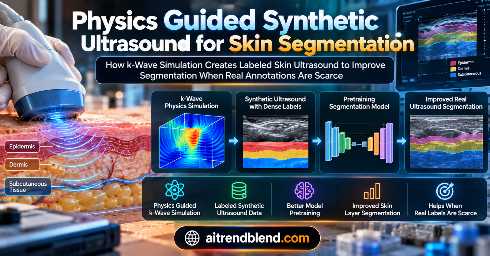
A dermatologist looking at a high frequency ultrasound scan of skin can read the layers the way a geologist reads rock strata. There is the bright epidermis at the surface, a dark band beneath it that clinicians call the subepidermal low echogenic band, then the dermis, the fat, the fascia, and the muscle below. Teaching a neural network to trace those same boundaries should be a solved problem by now. It is not, and the reason is almost embarrassingly simple. Nobody has labeled enough of the deeper layers for a model to learn them.
Key points
- Real skin ultrasound datasets label only the shallow structures, the epidermis and the dark band beneath it, so models cannot learn the dermis, fat, fascia, and muscle that dense analysis needs.
- A team at Yonsei University builds synthetic scans from a physics simulator instead of copying real image statistics, so every generated image arrives with an exact eight class label map for free.
- The pipeline assigns sound speed, density, and scattering to each skin layer, runs a k-Wave acoustic simulation, and exports a green channel image that matches the public real dataset.
- Pretraining on synthetic scans and then fine tuning on real data matched or beat real only training in three of four network architectures, with the best model reaching 83.40 percent mean Dice.
- The gains were modest, and the authors are candid about why, the synthetic speckle and reflector artifacts still do not fully match what a real scanner produces.
The annotation bottleneck nobody talks about
The problem runs deeper than it first appears. High frequency ultrasound, often shortened to HFUS, images the first few millimeters of skin at resolutions that ordinary clinical ultrasound cannot reach. Dermatologists use it to measure epidermal thickness, track inflammatory disease, watch skin aging, and plan aesthetic procedures. All of that depends on knowing where one layer ends and the next begins, which is exactly the kind of pixel by pixel task that deep learning segmentation was built for.
So where is the holdup? It lives in the labels. Building a supervised segmentation model needs images where an expert has already drawn the boundaries, and for skin ultrasound those expert drawings mostly stop at the surface. The widely used public resources annotate the epidermis and the subepidermal low echogenic band, the layer the field abbreviates as SLEB, and little else. Dense labels for the dermis, the subcutaneous fat, the fascia, and the muscle are rare to the point of near absence. That leaves researchers training models on a thin slice of the anatomy they actually care about, which is a strange place to be stuck given how mature segmentation methods have become.
The obvious escape is to make more data. The interesting question is how. One camp would reach for a generative model, a diffusion network or a generative adversarial network that learns the look of real ultrasound and produces convincing fakes. Those methods work, and the paper cites their success on echocardiography, breast ultrasound, and musculoskeletal imaging. But they share a quiet weakness. A model that learns to imitate images does not automatically know what each pixel represents, so the synthetic image still needs labeling, and the labeling problem returns through the back door. The authors of this work take a different road entirely.
Simulate the physics, get the labels for free
Here is where it gets interesting. Instead of teaching a network to mimic ultrasound pixels, the team from Yonsei University, Junkyung Ju, Kyungho Yoon, and Minwoo Shin, simulates the ultrasound from first principles. They build a multilayer acoustic model of skin, a stack of layers each given its own physical properties, and then they simulate how an ultrasound pulse would actually travel through it. Because they started from a known anatomical layout, they already know which pixel belongs to which layer. The label map is not something they draw afterward. It is an input to the simulation, so it comes out exact and free of human effort.
That inversion is the whole idea. A data driven generator learns images and struggles to produce labels. A physics guided simulator starts from labels and produces images. The paper makes the point plainly, that a useful synthetic dataset should preserve the anatomical ordering of skin layers while allowing controlled variation, which argues for a generator driven by acoustic layer maps rather than by image level style transfer alone.
Eight layers, each with its own acoustics
The simulator defines eight tissue classes, air, the coupling medium the probe sits in, epidermis, SLEB, dermis, subcutaneous tissue, fascia, and muscle. Every class is assigned two acoustic properties that govern how sound behaves inside it, a sound speed and a density, along with a scattering level that controls how grainy the tissue looks. These are not invented numbers. They are informed by reported acoustic properties of human skin and skin mimicking phantoms, so the epidermis carries a sound speed of about 1628 meters per second and a density near 1125 kilograms per cubic meter, while the dermis sits around 1578 meters per second, and the muscle near 1560. The dark SLEB is modeled as a low scatter band inserted in the upper skin, which is what gives it that characteristic hypoechoic darkness on a real scan.
| Layer | Sound speed (m/s) | Density (kg/m3) | Base scatter |
|---|---|---|---|
| Air near field | 1480 | 1000 | very low |
| Coupling medium | 1484 | 1002 | very low |
| Epidermis | 1628 | 1125 | moderate |
| SLEB | 1518 | 1015 | low scatter band |
| Dermis | 1578 | 1064 | high |
| Subcutaneous | 1556 | 1032 | moderate |
| Fascia | 1512 to 1558 | 978 to 1036 | thin sheet |
| Muscle | 1560 to 1565 | 1040 to 1045 | anisotropic |
Why layer boundaries show up at all
The physics that makes ultrasound imaging possible is worth pausing on, because it is what the simulator is quietly exploiting. Sound reflects at a boundary between two materials in proportion to the mismatch in their acoustic impedance, and impedance is just the product of density and sound speed.
When a pulse crosses from one layer to the next, the fraction of energy that bounces back is set by the reflection coefficient, the difference in impedance divided by the sum.
This one relation explains a great deal. The bright line at the top of the epidermis is a large impedance jump. The dermis looks grainy because it scatters strongly. The SLEB looks dark because it scatters weakly. By assigning sensible density and sound speed values to each class, the simulator gets these appearances to emerge on their own rather than being painted in by hand. The actual wave propagation is handled by k-Wave, an open acoustic simulation toolbox that models nonlinear ultrasound in heterogeneous media using a k space pseudospectral method, which is a well established tool in the acoustics community rather than something the authors had to invent.
The rendering choices that make it usable
Two production details matter more than they might seem. The simulation runs at a 20 megahertz configuration with 96 scan lines and exports images at 2067 by 1555 pixels over a 7.0 millimeter axial depth. That export size is not arbitrary. It is matched to the publicly available real HFUS skin images the team compares against, so the synthetic and real data can be used together without awkward resizing. The second choice is color. The public real images are distributed in a green channel display format, so the simulator renders its output the same way, deriving a green channel image from the simulated signal so that a model pretrained on synthetic data sees the same visual format it will later meet in the real fine tuning stage. The raw integer mask is kept separately, so the display choice never contaminates the labels.
Making the data vary without breaking the labels
A single fixed skin geometry would teach a model almost nothing, so the generator introduces three families of variation. Layer thickness variation changes the relative depth of the superficial and deeper layers from sample to sample. Boundary shape variation perturbs the morphology and smoothness of the interfaces, allowing non flat epidermal, SLEB, and dermal boundaries instead of tidy horizontal lines. Tissue heterogeneity variation alters the dermal scattering, the subcutaneous texture, the visibility of the fascia, and the muscle texture.
On top of those anatomical changes, the pipeline applies label preserving image augmentation, the familiar rotations and similar transforms, after generation. The separation is deliberate and it is one of the cleaner ideas in the method. Structural variation changes the simulated anatomy before the image is formed, so the label map changes with it and stays correct. Augmentation changes the exported image and its mask together after generation. Keeping anatomy level diversity distinct from training time appearance augmentation means the two never interfere, and the mask is always right no matter which knob was turned.
In the released dataset, 200 original synthetic samples are produced from parent simulations along with their paired variants. For the downstream test, the eight class masks are folded down into a three class target space, other, epidermis, and SLEB, so that the synthetic supervision lines up exactly with the public real annotations, which only cover those two structures plus background. The full eight class labels remain available for anyone who wants to study the deeper layers, but the head to head evaluation stays on the ground where real labels exist.
A data driven generator learns to imitate images and then still needs someone to label them. A physics guided simulator starts from the labels and renders the image, which is the difference between borrowing appearance and building anatomy. Reading of the paper’s motivation
Does synthetic pretraining actually help
A generator is only as good as what it does for a real task, so the real test is downstream. The team took four segmentation architectures that can be trained from scratch, a fresh SegUNet, a U-Net, a DeepLabV3+, and a SegFormer, and ran each one two ways. The first way was real only, training on the public Mendeley HFUS dataset alone. The second way was synthetic pretraining followed by real fine tuning, one hundred epochs on the synthetic data first and then up to three hundred epochs on the real data. A previously released SegUNet served as a contextual reference point. All real experiments used the same 64 by 128 region of interest inputs, the same split, and the same Dice and intersection over union implementation, so the only thing that changed was whether synthetic pretraining happened.
The numbers below report class wise Dice for the epidermis and SLEB, then the mean Dice and mean intersection over union averaged over the two classes.
| Model | Setting | Epi Dice | SLEB Dice | Mean Dice | Mean IoU |
|---|---|---|---|---|---|
| Released SegUNet | released model | 78.14 | 79.51 | 78.82 | 65.05 |
| Fresh SegUNet | real only | 87.52 | 77.75 | 82.64 | 70.71 |
| Fresh SegUNet | synth then real | 87.91 | 78.90 | 83.40 | 71.79 |
| U-Net | real only | 87.61 | 76.64 | 82.13 | 70.04 |
| U-Net | synth then real | 87.79 | 78.39 | 83.09 | 71.35 |
| DeepLabV3+ | real only | 83.00 | 77.56 | 80.28 | 67.14 |
| DeepLabV3+ | synth then real | 82.98 | 77.06 | 80.02 | 66.80 |
| SegFormer | real only | 84.67 | 80.35 | 82.51 | 70.28 |
| SegFormer | synth then real | 85.42 | 79.91 | 82.66 | 70.54 |
The pattern is consistent without being dramatic. Synthetic pretraining raised the mean Dice and mean intersection over union in three of the four trainable architectures. The fresh SegUNet gained the most in absolute terms, climbing from 82.64 to 83.40 mean Dice and from 70.71 to 71.79 mean intersection over union, the best result in the table. The U-Net improved by nearly a full point of mean Dice. The SegFormer improved slightly. Only the DeepLabV3+ went the other way, slipping by about a quarter of a point, which is small enough to sit inside ordinary run to run noise but honest enough that the authors report it rather than hiding it.
The Dice coefficient and the intersection over union that anchor these results are the standard overlap measures for segmentation, defined for a predicted region and a ground truth region as
What matters here is not a leaderboard record. The authors say so directly, that the purpose was to test whether synthetic HFUS images provide transferable supervision, not to establish a new best in segmentation. Read that way, the result is quietly important. The synthetic images did not just fail to hurt real performance, which would already be a useful finding. They helped in most cases, which means the physics simulator is encoding layer structured cues that a real segmentation model can reuse.
Clinical translation gap
None of this reaches a clinic tomorrow, and it is worth being clear about the distance involved. The evaluation lives entirely on a single public research dataset, with region of interest crops of 64 by 128 pixels, and the real labels cover only two structures, the epidermis and the SLEB. The deeper layers that the simulator can label, the dermis and fat and fascia and muscle, have no real annotations to test against, so their accuracy on real scanner images is simply unknown. The paper is careful to present the expanded multilayer label space as a capability of the generator, demonstrated through the dense synthetic masks, rather than as a validated real domain result.
There is also the matter of who acquired the data and how. HFUS images vary with the probe, the operator, the coupling, and the patient, and a method validated on one public collection has not been shown to hold up across scanners, clinics, or skin types. A tool that measures epidermal thickness or tracks an inflammatory condition would need prospective testing on the population it is meant to serve, under the regulatory pathway for clinical software, before any of its numbers should inform a decision. Nothing in this paper claims otherwise. The authors frame the work as an initial validation of the usability of synthetic HFUS, not a solution to real domain segmentation, and that framing is the right one to carry forward.
Honest limitations
The improvements were modest, and the paper does not dress them up. The most likely reason is that the synthetic images still differ from real scanner acquired HFUS in appearance. Speckle distribution, attenuation behavior, boundary sharpness, and reflector artifacts do not yet match what a real transducer produces, and those differences plausibly explain both the size of the gains and why they varied by architecture. In particular the authors flag overly strong reflector artifacts near the SLEB to dermis transition as something to reduce before the multilayer labels can be trusted on real data.
Cost is a real constraint too, and it cuts against the method’s main advantage. A learned generator, once trained, can sample new images cheaply. Each physics based sample here requires a full wave equation simulation, which is computationally expensive. Simply generating more samples from the same simulator would preserve the same appearance bias rather than closing the gap with real images, so scaling the dataset is not a free lever. The dataset used in the study is small by modern standards, 200 parent synthetic samples plus variants, and the real evaluation set is a single public collection, so the sample sizes on both sides are limited and the results should be read as a proof of transfer rather than a precise measurement of how much synthetic data helps.
Dataset bias deserves its own mention. Because the real labels exist only for the epidermis and SLEB, every quantitative claim about real performance is confined to those two classes. The three class mapping used for evaluation was chosen precisely so the synthetic supervision would line up with what the real dataset can check, which is sound methodology, but it also means the deeper layers ride along untested. Generalization beyond this one dataset, this one display format, and this one region of interest size is not established, and the authors do not claim it is.
Why the approach still matters
Step back from the modest deltas and the larger picture is more encouraging than the numbers alone suggest. The result that synthetic pretraining did not degrade real performance, and usually improved it, tells us the generated images carry transferable anatomical and textural priors. They are not merely plausible to the eye. They encode layer structured information that real segmentation models can pick up and reuse, which is a stronger claim than visual realism and a more useful one.
The deeper contribution is the dense multilayer labels the simulator can produce beyond what any real dataset offers. Real annotations stop at the epidermis and SLEB. The simulator hands out labels for the dermis, subcutaneous tissue, fascia, and muscle as well, at no annotation cost. Even if those deeper labels cannot yet be validated against real scans, they open a path toward multilayer skin analysis that the annotation bottleneck had closed off. Reducing the appearance gap, especially those reflector artifacts near the SLEB to dermis boundary, is the concrete next step the authors name for turning this from a promising prior into reliable multilayer supervision.
Conclusion
This paper is a clean example of solving a data problem by changing the question. The field had been asking how to label more skin ultrasound images, a slow and expensive task that experts can barely keep up with for the shallow layers, let alone the deep ones. The Yonsei team asked instead how to generate images that come pre labeled, and the answer was to simulate the acoustics rather than imitate the pixels. When you build the anatomy first and render the ultrasound second, the segmentation mask is no longer a separate chore. It falls out of the generation process, exact and complete for every layer.
The conceptual shift is from appearance to structure. A generative model that learns the look of real ultrasound captures its style but not its meaning, so it cannot supply labels without human help. A physics simulator that assigns sound speed, density, and scattering to each tissue and then propagates a wave through the stack captures the mechanism that produces the image, and the mechanism is exactly what ties a pixel to a layer. That is why the synthetic images transferred at all. They were built from the same physical relationships that give real scans their structure.
The evidence supports a careful claim rather than a sweeping one. Across four architectures, synthetic pretraining followed by real fine tuning matched or improved real only training in three, and reached 83.40 percent mean Dice at its best. Those are real gains, and the fact that they held across most architectures rather than a single lucky one is what makes them credible. They are also small, and the authors correctly attribute that to a residual appearance gap between simulated and scanner acquired images that more samples alone will not close.
The honest limitations keep the work grounded. Real validation covers only two of eight layers, the dataset is modest and single source, each synthetic sample is expensive to compute, and reflector artifacts near the SLEB to dermis transition still betray the simulation. None of these is fatal, and each points to a specific improvement rather than a dead end. Better acoustic modeling of speckle and attenuation, richer phantom variation, and real labels for the deeper layers would all move the method forward.
For anyone working where labeled medical images are scarce, which is most of medical imaging, the transferable lesson is the appealing part. If you can write down the physics that forms your image, you may not need to wait for annotations at all. You can simulate the thing you want a model to learn, keep the labels exact because you authored them, and let a real dataset do the final tuning. Skin ultrasound is a hard test case precisely because its layers are thin and its appearance is noisy, so a method that shows transfer here is worth watching as it moves to other imaging problems with the same shortage of labels.
Reference implementation in Python
The code below is a compact, runnable sketch of the ideas in the paper. It builds a layered acoustic skin phantom with the three families of variation, derives a reflectivity map from impedance gradients, renders a simple B mode style image by blurring the reflectivity and adding speckle, and exports a paired dense mask. It then defines a small U-Net and runs a synthetic pretraining plus real fine tuning loop, with a smoke test on dummy tensors. The true pipeline uses k-Wave for full wave equation simulation, which needs its own toolbox, so this stands in with a convolution based approximation for study purposes.
# synthetic_hfus.py
# Study reference for physics guided synthetic HFUS ideas. Not the authors'
# k-Wave pipeline. Approximates B mode rendering with a convolution model so it
# runs anywhere. Ends with a smoke test on dummy data.

import numpy as np
import torch
import torch.nn as nn
import torch.nn.functional as F

# eight class label ids, matching the paper's target space
CLASSES = {
    "air": 0, "coupling": 1, "epidermis": 2, "sleb": 3,
    "dermis": 4, "subcut": 5, "fascia": 6, "muscle": 7,
}
# sound speed c (m/s), density rho (kg/m3), scatter strength per class
ACOUSTIC = {
    "air":       (1480, 1000, 0.00002),
    "coupling":  (1484, 1002, 0.0002),
    "epidermis": (1628, 1125, 0.010),
    "sleb":      (1518, 1015, 0.001),   # low scatter band, looks dark
    "dermis":    (1578, 1064, 0.022),   # strong scatter, looks bright and grainy
    "subcut":    (1556, 1032, 0.0062),
    "fascia":    (1535, 1007, 0.004),
    "muscle":    (1562, 1042, 0.006),
}


def build_phantom(h=128, w=128, rng=None):
    """Build a layered label map with the three families of variation.
    Returns the dense mask, plus sound speed and density maps."""
    rng = rng or np.random.default_rng()
    mask = np.zeros((h, w), dtype=np.int64)
    # base fractional thickness per layer, then thickness variation
    order = ["coupling", "epidermis", "sleb", "dermis", "subcut", "fascia", "muscle"]
    base = np.array([0.12, 0.06, 0.05, 0.30, 0.20, 0.05, 0.22])
    thick = base * (1.0 + 0.25 * rng.standard_normal(base.shape))  # thickness variation
    thick = np.clip(thick, 0.02, None)
    thick = thick / thick.sum()
    edges = np.cumsum(thick) * h
    # boundary shape variation, a smooth wavy offset per column
    phase = rng.uniform(0, 2 * np.pi)
    amp = rng.uniform(0, 4.0)
    wob = amp * np.sin(np.linspace(0, 3 * np.pi, w) + phase)
    for x in range(w):
        prev = 0
        for name, e in zip(order, edges):
            top = int(prev + wob[x])
            bot = int(e + wob[x])
            mask[max(0, top):max(0, bot), x] = CLASSES[name]
            prev = e
    # build sound speed and density maps from the label map
    c_map = np.zeros((h, w)); rho_map = np.zeros((h, w)); sc_map = np.zeros((h, w))
    for name, cid in CLASSES.items():
        c, rho, sc = ACOUSTIC[name]
        sel = mask == cid
        # tissue heterogeneity variation, per pixel scatter jitter
        c_map[sel] = c
        rho_map[sel] = rho
        sc_map[sel] = sc * (1.0 + 0.4 * rng.standard_normal(sel.sum()))
    return mask, c_map, rho_map, np.clip(sc_map, 0, None)


def render_bmode(c_map, rho_map, sc_map, rng=None):
    """Approximate a B mode image. Reflectivity comes from impedance gradients
    Z = rho * c, plus scatter texture, blurred by a point spread function."""
    rng = rng or np.random.default_rng()
    Z = rho_map * c_map
    # axial impedance gradient gives specular boundary reflections
    dZ = np.zeros_like(Z)
    dZ[1:, :] = np.abs(Z[1:, :] - Z[:-1, :]) / (Z[1:, :] + Z[:-1, :] + 1e-6)
    speckle = sc_map * np.abs(rng.standard_normal(Z.shape))  # diffuse scatter
    reflect = 6.0 * dZ + speckle
    # point spread function, wide laterally and narrow axially
    img = _blur(reflect, ksize_ax=3, ksize_lat=7)
    # attenuation with depth, then log compression like real B mode
    depth = np.linspace(1.0, 0.5, img.shape[0])[:, None]
    img = img * depth
    img = np.log1p(40.0 * img)
    img = img / (img.max() + 1e-6)
    return img.astype(np.float32)


def _blur(x, ksize_ax=3, ksize_lat=7):
    t = torch.tensor(x)[None, None].float()
    k = torch.ones(1, 1, ksize_ax, ksize_lat) / (ksize_ax * ksize_lat)
    pad = (ksize_lat // 2, ksize_lat // 2, ksize_ax // 2, ksize_ax // 2)
    return F.conv2d(F.pad(t, pad, mode="reflect"), k)[0, 0].numpy()


def to_three_class(mask):
    """Map eight class labels to other, epidermis, SLEB for the real task."""
    out = np.zeros_like(mask)
    out[mask == CLASSES["epidermis"]] = 1
    out[mask == CLASSES["sleb"]] = 2
    return out


class TinyUNet(nn.Module):
    """A small U-Net for the three class segmentation head."""
    def __init__(self, n_classes=3, ch=32):
        super().__init__()
        self.e1 = self._block(1, ch)
        self.e2 = self._block(ch, ch * 2)
        self.b = self._block(ch * 2, ch * 4)
        self.d2 = self._block(ch * 4 + ch * 2, ch * 2)
        self.d1 = self._block(ch * 2 + ch, ch)
        self.out = nn.Conv2d(ch, n_classes, 1)
        self.pool = nn.MaxPool2d(2)

    def _block(self, ci, co):
        return nn.Sequential(
            nn.Conv2d(ci, co, 3, padding=1), nn.BatchNorm2d(co), nn.ReLU(True),
            nn.Conv2d(co, co, 3, padding=1), nn.BatchNorm2d(co), nn.ReLU(True))

    def forward(self, x):
        e1 = self.e1(x)
        e2 = self.e2(self.pool(e1))
        b = self.b(self.pool(e2))
        d2 = self.d2(torch.cat([F.interpolate(b, scale_factor=2), e2], 1))
        d1 = self.d1(torch.cat([F.interpolate(d2, scale_factor=2), e1], 1))
        return self.out(d1)


def dice_score(logits, target, n_classes=3, eps=1e-6):
    pred = logits.argmax(1)
    scores = []
    for c in range(1, n_classes):  # skip background class 0
        a = (pred == c).float(); b = (target == c).float()
        inter = (a * b).sum()
        scores.append((2 * inter + eps) / (a.sum() + b.sum() + eps))
    return torch.stack(scores).mean()


def synth_batch(n=4, h=128, w=128, rng=None):
    rng = rng or np.random.default_rng(0)
    imgs, masks = [], []
    for _ in range(n):
        m, c, rho, sc = build_phantom(h, w, rng)
        imgs.append(render_bmode(c, rho, sc, rng))
        masks.append(to_three_class(m))
    x = torch.tensor(np.stack(imgs))[:, None]
    y = torch.tensor(np.stack(masks))
    return x, y


def train_step(model, opt, x, y):
    model.train(); opt.zero_grad()
    loss = F.cross_entropy(model(x), y)
    loss.backward(); opt.step()
    return loss.item()


def smoke_test():
    torch.manual_seed(0)
    model = TinyUNet()
    # phase 1, synthetic pretraining
    opt = torch.optim.SGD(model.parameters(), lr=1e-3, momentum=0.9, weight_decay=5e-4)
    for step in range(3):
        x, y = synth_batch(4)
        print(f"synth pretrain step {step} loss {train_step(model, opt, x, y):.3f}")
    # phase 2, real fine tuning stands in with a fresh dummy batch and lower lr
    opt = torch.optim.SGD(model.parameters(), lr=1e-4, momentum=0.9, weight_decay=5e-4)
    xr = torch.randn(2, 1, 128, 128)
    yr = torch.randint(0, 3, (2, 128, 128))
    print(f"real finetune loss {train_step(model, opt, xr, yr):.3f}")
    x, y = synth_batch(4)
    with torch.no_grad():
        print(f"synthetic mean Dice {dice_score(model(x), y).item():.3f}")
    n = sum(p.numel() for p in model.parameters())
    print(f"parameter count {n/1e6:.3f} M")


if __name__ == "__main__":
    smoke_test()
Running the smoke test prints the synthetic pretraining losses, a real fine tuning step, a mean Dice on held out synthetic samples, and the parameter count. It demonstrates the two phase recipe in miniature, synthetic first and real second, on a phantom that follows the same layer ordering and variation families the paper describes.
Frequently asked questions
What is high frequency ultrasound used for in skin imaging?
It provides high resolution views of the first few millimeters of skin, which clinicians use to measure epidermal thickness, monitor inflammatory disease, study skin aging, and plan aesthetic procedures. Automated layer segmentation supports those measurements.
Why not just use a generative model to make synthetic ultrasound?
A generative model learns to imitate the look of real images but does not automatically know which pixel belongs to which layer, so the synthetic images still need labeling. The physics simulator starts from a known anatomical layout, so the dense label map comes out exact and free.
How does the simulator decide what each layer looks like?
It assigns every tissue class a sound speed, a density, and a scattering level, then simulates how an ultrasound pulse travels through the stack with the k-Wave toolbox. Reflections at layer boundaries and scattering inside layers produce the familiar appearance without any of it being drawn by hand.
Did synthetic pretraining actually improve real segmentation?
Yes, in three of the four network architectures tested. Pretraining on synthetic data and fine tuning on real data raised mean Dice and mean intersection over union for the fresh SegUNet, the U-Net, and the SegFormer, with the best model reaching 83.40 percent mean Dice, while DeepLabV3+ changed by a negligible amount.
Is this system ready for clinical use?
No. It is a research method validated on a single public dataset, with real labels for only two of the eight layers, and it has not undergone prospective clinical testing or regulatory review. It should be read as an early demonstration of transfer, not as an approved tool.
What are the main limitations of the approach?
Synthetic images still differ from real scanner images in speckle, attenuation, boundary sharpness, and reflector artifacts, which likely explains the modest gains. Each physics based sample is expensive to compute, the datasets are small, and deeper layer accuracy on real scans remains untested.
Read the full paper and browse the released code and dataset.
Read the paper on arXiv Code and data on GitHub