
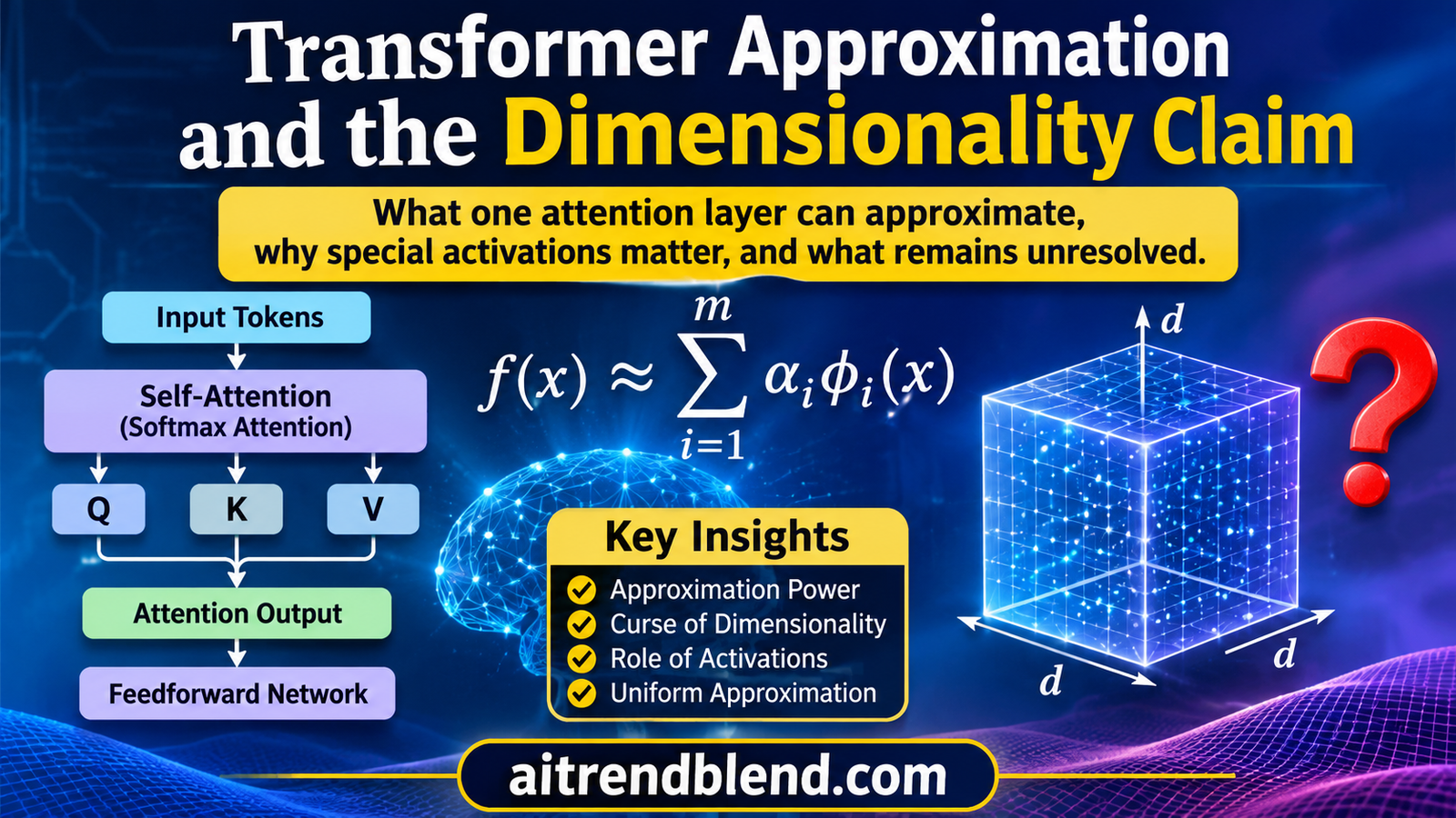
A researcher adds more input variables to a regression model and watches the required approximation grid become unmanageable. Each variable adds another axis along which the target can change. A new Transformer theorem offers a striking alternative. One attention layer can be enough to represent a broad family of such targets with favorable accuracy exponents. The immediate question is what the rest of the architecture must do to make that possible.
- The paper proves existence of Transformer approximations for Hölder continuous functions on a fixed matrix domain.
- The construction needs one softmax attention layer with one head, surrounded by carefully designed feedforward blocks.
- Special activations, including floor in the uniform approximation result, are essential to the reported bounds.
- The dimension leaves the exponent of approximation accuracy in selected size bounds, but still affects explicit widths, depths and numerical encoding.
- A separate experiment trains a model with five heads on a two variable synthetic target.
- Representation size, parameter precision, optimization and generalization remain separate questions.
What the Transformer dimensionality theorem establishes
Yuling Jiao, Yanming Lai, Yang Wang and Bokai Yan develop the argument in their JMLR study of Transformer approximation. The published paper appears in volume 27 as article 50 in 2026. Its main object is a mathematical sequence transformation. An input matrix has a fixed number of tokens and a fixed number of coordinates per token. The output has the same shape.
The authors are affiliated with Wuhan University, Hong Kong Polytechnic University, the University of Hong Kong and the Hong Kong University of Science and Technology. Their contribution connects approximation results for feedforward networks to a Transformer construction through a version of the Kolmogorov Arnold representation theorem. A translation technique lets a shared feedforward operation act differently on different token positions.
The useful reading is architectural. It identifies a sufficient way to divide the work between local coordinate processing and global token aggregation. It does not establish that an ordinary language model discovers this division when trained on text. Nor does it show that a vision model can discard most of its attention layers without losing accuracy.
This analysis belongs to the Vision Transformers and Attention collection within Machine Learning. Its angle is the accounting behind expressivity. Which resource becomes smaller, which assumptions permit that reduction, and which costs remain outside the theorem?
The curse concerns the accuracy exponent
Imagine approximating a function by dividing each input coordinate into small intervals. A grid that is manageable along one coordinate can become enormous when every coordinate gets its own independent partition. Smoothness limits how quickly the target changes, but a generic multivariate target can still require many cells.
The paper studies functions with Hölder regularity. If two inputs are close in the largest coordinate difference, each output coordinate must also be close, according to a power law. The exponent lies at most at one in the stated definition. The constant controls how much variation is permitted.
Here the total input dimension is \(D=dn\). The domain is compact and fixed. The result allows each output coordinate to depend on the whole input, rather than assuming that each token can be processed independently. That dependence is exactly why the construction needs some communication between columns.
In several conventional approximation bounds summarized by the paper, width grows like a power of inverse accuracy whose exponent contains the input dimension. The new construction removes that dimension from selected accuracy exponents by expanding the activation family. This is a statement about a particular representation model. Comparing it to a restricted ReLU network without recording that change would hide a central assumption.
The distinction complements our discussion of ReLU representations and dimensionality. Different function classes, norms and representation mechanisms support different claims. A favorable exponent under one collection of assumptions does not transfer automatically to another collection.
How many resources does the first theorem require?
Theorem 6 gives uniform approximation. Every permitted input and every output coordinate must satisfy the error tolerance. Its first construction combines ReLU and floor activations. The initial feedforward block doubles the token channel dimension before attention. A final block converts the resulting representation into the output.
The initial block has width \(3dn\) and depth determined by a logarithm of inverse accuracy, divided by the smoothness exponent. For the ReLU and floor decoder, the stated depth is \(7dn-2\). Its width includes dimension dependent factors and an accuracy power \(2/\beta\), together with a logarithmic factor involving the outer function range.
These asymptotic expressions describe accuracy dependence with other quantities fixed. They do not say that width and depth are independent of token count or embedding dimension. In particular, calling the decoder depth constant refers to accuracy, not to the product of token count and coordinate count.
Other activation families reduce the decoder’s accuracy dependence further. Adding an exponential activation gives a logarithmic width option. Allowing a suitable analytic activation or the paper’s reciprocal activation gives decoder widths proportional to the output coordinate dimension. The initial encoding block remains part of the model, so constant decoder width should not be mistaken for constant total construction size under arbitrary changes of dimension.
| Result family | Error control | Important activation assumption | What to retain |
|---|---|---|---|
| Theorem 6 first option | Uniform over the input domain | ReLU and floor | Accuracy exponent in selected width bound does not contain total input dimension |
| Theorem 6 smaller decoder options | Uniform over the input domain | Floor with exponential or other specified activations | Smaller decoder size uses a richer computational primitive |
| Theorem 7 | Integrated coordinate error | ReLU encoder with special decoder activations | A small exceptional input region can be tolerated |
| Section 4 experiment | Mean squared error on sampled points | Several activation combinations | Training evidence on a small synthetic task is separate from the existence theorem |
The favorable exponent is real within the stated model. Reading it responsibly means carrying the activation family, error norm, dimension factors and precision assumptions alongside the size expression.
The representation hides coordinates in digits
The construction uses a representation theorem developed through a Cantor set encoding. A coordinate’s binary digits are placed into widely separated positions of a ternary expansion. Different coordinates occupy different digit positions, so their contributions can be summed without losing their identities in exact arithmetic.
For a flattened input of dimension \(D\), the paper introduces a truncated inner encoding. The digit \(a_j^x\) is the selected binary digit of a scalar input. The finite truncation uses a precision parameter \(K\).
Each output coordinate then has its own outer function evaluated on the shared scalar code. The full representation theorem concerns an infinite encoding. The approximation proof replaces it with a finite one and controls the resulting error using target regularity.
This is a sophisticated address system. The encoder assigns input configurations to locations in a scalar domain, and the decoder returns the required outputs for those locations. Reducing the number of intermediate coordinates does not imply that the information content of the target has vanished. Much of the difficulty moves into the numerical arrangement of that address system and the function that reads it.
The relevant version of the representation theorem transfers regularity to the outer function while allowing discontinuities in the inner function. Dyadic rationals require a consistent choice of binary representation. The paper discusses this explicitly. A reader should therefore resist assuming that every intermediate mapping behaves like a smooth learned embedding.
One attention head supplies the global sum
The role of attention is surprisingly modest. Once each token contains its properly weighted coordinate contribution, the model needs to sum those contributions across token positions. Uniform softmax weights can supply an average, and a linear scaling can turn that average into a sum.
The actual construction must also accommodate the residual connection in its attention definition. Extra channels and linear maps allow the desired aggregate to be recovered. The proof is therefore more specific than replacing an arbitrary attention layer with average pooling in an existing trained network.
The theoretical architecture omits layer normalization. Its feedforward blocks also do not include the usual feedforward residual connection. Those design choices are explicit in the preliminaries. Treating the model as identical to a standard encoder block would erase differences that matter to the proof.
The paper’s point is that elaborate content dependent attention is not necessary for this existence result. Information from different columns still must interact. A token wise feedforward block cannot perform that cross column sum on its own under the specified matrix operations.
“even using only summation across columns”Jiao, Lai, Wang and Yan, discussing the sufficient token interaction in their construction.
This perspective is distinct from how optimization changes attention token selection. That question concerns which attention behavior training favors in a simplified model. The present result describes a deliberately constructed sufficient representation. Existence and selection require different arguments.
Translation gives a shared network a sense of position
A shared feedforward function applies the same mapping to every token. Yet the encoding needs different coordinate weights for different positions. The authors resolve this by translating token domains into separate intervals before applying a shared function.
In their illustrative example, later columns receive offsets of two and four. Inputs originally lying in the same unit interval then occupy disjoint translated intervals. One shared function can implement different prescribed behavior on those separated parts of its domain.
The decoder uses a related idea. Each output position receives a translated version of the shared encoded value, letting a common feedforward map return the position appropriate output. The model definition permits bias matrices with different columns, which supports this position dependent operation.
This matters for symmetry. A shared network with no position information has restrictions imposed by token permutation symmetry. The construction should not be read as proving approximation of every ordered sequence transformation while preserving that restriction. The translations provide position information through the allowed bias structure.
Our guide to video Transformer design choices also separates token processing from position encoding. Here that separation is part of a proof mechanism, rather than an empirical comparison of video architectures. The shared lesson is to inspect how token identity enters before drawing conclusions about attention alone.
Uniform error and integrated error protect different things
Theorem 7 controls an integrated error for finite \(p\). It uses a ReLU encoding that agrees with the desired truncated map outside a small flawed region. The proof bounds the error on the good region and separately bounds the contribution from the exceptional region.
The measure here is the domain’s Lebesgue measure. It is not an arbitrary deployment distribution. A small volume region could receive substantial probability under a different input distribution. Transferring the integrated guarantee would therefore require additional information about how inputs are distributed.
Likewise, sampled mean squared error does not certify the uniform guarantee. A test set can miss narrow regions where a discontinuous encoder changes rapidly. This is especially relevant when the mechanism deliberately uses tiny intervals or closely packed numerical addresses.
The paper bounds the bad region’s contribution using its measure and a bound on the output. That is an analytically useful strategy, but it does not make the region irrelevant to every application. The choice of norm belongs in the headline interpretation of the theorem.
Before using an approximation claim, ask what receives protection. A uniform bound covers every input. An integrated bound controls average error under its stated measure. A finite test set measures only the sampled inputs.
The training experiment is informative and deliberately small
Section 4 tests a two component target on the unit square. Both components are sums of sine functions with different frequencies and coefficients. The target is explicit, so independent training and test examples can be sampled without label noise or annotation uncertainty.
The training set contains 10000 uniformly sampled points and the test set contains 2000. Both feedforward blocks have width 50. Their depths are five and three, and the attention layer has five heads. The experiment includes dropout in the first block and gradient clipping during optimization.
| Reported setting | Value | Interpretation |
|---|---|---|
| Input domain | Unit square | Two variable experiment |
| Training and test samples | 10000 and 2000 | Independent sampled evaluations |
| Feedforward width | 50 in both blocks | Finite practical network |
| Feedforward depths | Five and three | Architecture differs from an arbitrary theorem construction |
| Attention heads | Five | Does not empirically test the one head sufficiency claim |
| Optimizer and batch size | Adam and 64 | Mean squared error objective |
| Training schedule | 500 epochs | Initial learning rate 0.001 reduced by a factor of 0.1 every 200 epochs |
Figure 2 plots training and test losses for several activation combinations. It provides evidence that these choices can be trained in the illustrated setting. The paper does not supply a tabulated collection of final losses, uncertainty intervals across seeds or a scaling study across increasing input dimensions. Reading precise numerical advantages from the plotted lines would overstate what is reported.
The practical gap is therefore specific. A two variable training demonstration does not establish favorable sample or optimization complexity for arbitrary dimension. It also does not show that the exact bit encoding and memorization construction is recovered by Adam.
Precision and learning are still expensive questions
The illustrative construction rescales the scalar encoding by a power of three involving both dimension and truncation precision. That exposes an important resource outside neuron count. The numerical range and the spacing between encoded values change as the construction becomes more demanding.
Real arithmetic permits a parameter to carry information at arbitrary precision. Hardware uses finite representations. Consequently, a small parameter count can coexist with a difficult requirement on parameter precision or intermediate dynamic range. The paper’s size theorem should not be advertised as a bit complexity bound.
Floor has zero derivative almost everywhere in ordinary automatic differentiation. A literal implementation of the discontinuous encoding is therefore a poor default training component for gradient descent. Replacing it with a surrogate derivative changes the optimization procedure and requires its own justification. The code below makes no such replacement.
Exponential and reciprocal activations create other numerical concerns, including extreme values and proximity to singularities. These observations identify implementation questions. They do not invalidate the existence theorem, which operates under its own mathematical definitions.
Generalization remains a separate limitation. The authors explicitly warn that highly expressive unconventional activations can bring high complexity and large generalization error. They do not claim minimax optimal regression learning rates for the constructed family. Our discussion of generalization bounds for shallow ReLU networks explores why a representation result alone is insufficient to settle statistical performance.
What a useful next experiment would measure
A stronger practical investigation would vary total input dimension while keeping the target family and error definition explicit. It would separate the network size required by the construction from the size selected by training, and would record parameter precision alongside accuracy. These are proposed evaluation choices, not results from the paper.
It would also compare ordinary activations against the special activation families under the same training budget. Different choices can change both expressivity and numerical conditioning. Multiple seeds and complete hyperparameter reporting would help distinguish an architecture effect from an unusually favorable run.
Uniform error would require a separate assessment from average test loss. For a small domain, a dense diagnostic grid could reveal missed regions, although even that grid is not a proof over every point. For larger domains, targeted probes near encoding boundaries could expose failure modes that random sampling overlooks.
The most useful research question is how much of this constructive mechanism survives constraints on weight magnitude, precision and trainability. Such constraints could turn the theorem into a sharper guide for practical architectures. The current paper supplies a framework for asking that question, rather than its final answer.
A representation result with a clear boundary
The achievement is a constructive route from Hölder functions to Transformers whose selected accuracy exponents avoid the total input dimension. One softmax attention layer can perform the required global aggregation when the surrounding networks implement the right encoding and decoding.
The conceptual shift is in the division of labor. Attention need not carry every complicated interaction directly. A carefully arranged representation can make a simple token sum sufficient, with the remaining difficulty assigned to local feedforward operations.
The translation technique is valuable beyond this particular target class. It offers a way to adapt different token functions into one shared operation over separated domains. Any transfer to another function space, architecture or task still needs its own approximation and complexity argument.
The remaining limits are substantial and concrete. Special activations, position dependent biases, exact arithmetic reasoning and a small empirical demonstration leave optimization efficiency, statistical generalization and numerical robustness unresolved. None of those questions can be settled by counting attention heads alone.
Future work can make the bridge more practical by charging for precision, restricting activations and testing dimension dependent learning behavior. For now, the paper changes what a Transformer can be shown to represent. The next challenge is making that representation affordable to learn.
Complete PyTorch experiment companion
The reference below provides custom attention and feedforward layers, the full model, the paper’s synthetic target, mean squared error training, evaluation and a runnable smoke test. It includes a small diagnostic of the truncated digit encoding. That diagnostic is discontinuous and does not supply the theorem’s outer memorization network.
This is an editorial experiment companion. Section 4 does not fully specify activation placement, dropout probability, clipping threshold or every channel choice. The code labels those choices explicitly and uses a smooth mixture of ReLU, sine and hyperbolic tangent for training. It does not reproduce the published curves, activation variants or quantitative theorem construction. The default two epochs provide a smoke run. Set the epoch argument to 500 for the reported schedule length.
Python syntax and independent numerical checks of the target, encoding and attention aggregation passed. PyTorch was unavailable in the execution environment, so the runtime smoke test remains unexecuted and no training result is claimed. The sampled maximum error returned by evaluation is not a uniform certificate.
"""Editorial reference for Jiao et al., JMLR 27(50), 2026.
Not an implementation of the theorem's finite-memory construction.
A differentiable, five-head experiment companion with explicit choices.
Requires Python 3.10+ and PyTorch. Run --epochs 2 for a smoke run.
"""
import argparse
import math
import torch
from torch import nn
from torch.utils.data import DataLoader, TensorDataset


class MixedActivation(nn.Module):
    """Illustrative smooth combination, not the paper's unspecified layout."""
    def forward(self, x):
        return (torch.relu(x) + torch.sin(x) + torch.tanh(x)) / 3


class TokenBlock(nn.Module):
    """Depth counts affine maps. No feedforward residual or normalization."""
    def __init__(self, incoming, outgoing, width, depth, dropout=0.0):
        super().__init__()
        layers = []
        for k in range(depth - 1):
            layers += [nn.Linear(incoming if k == 0 else width, width),
                       MixedActivation()]
            if dropout:
                layers.append(nn.Dropout(dropout))
        layers.append(nn.Linear(width, outgoing, bias=False))
        self.net = nn.Sequential(*layers)

    def forward(self, x):
        return self.net(x)


class ResidualAttention(nn.Module):
    """Unscaled dot products as defined in the theoretical paper."""
    def __init__(self, channels, heads, head_size):
        super().__init__()
        self.heads, self.head_size = heads, head_size
        self.q = nn.Linear(channels, heads * head_size, bias=False)
        self.k = nn.Linear(channels, heads * head_size, bias=False)
        self.v = nn.Linear(channels, heads * head_size, bias=False)
        self.out = nn.Linear(heads * head_size, channels, bias=False)

    def forward(self, x):
        batch, tokens, _ = x.shape
        def split(layer):
            return layer(x).reshape(batch, tokens, self.heads,
                                    self.head_size).transpose(1, 2)
        q, k, v = split(self.q), split(self.k), split(self.v)
        weights = torch.softmax(q @ k.transpose(-2, -1), dim=-1)
        mixed = (weights @ v).transpose(1, 2).reshape(batch, tokens, -1)
        return x + self.out(mixed)


class ExperimentCompanion(nn.Module):
    """Two scalar tokens. Translation distinguishes their input coordinates.

    Paper reports widths 50, depths 5/3, five heads, dropout in F1.
    Channel count 10, head size 2, dropout .1 and this activation layout
    are editorial choices, not recovered author settings.
    """
    def __init__(self):
        super().__init__()
        self.register_buffer('translation', torch.tensor([0., 2.]).view(1, 2, 1))
        self.first = TokenBlock(1, 10, 50, 5, dropout=0.1)
        self.attention = ResidualAttention(10, 5, 2)
        self.last = TokenBlock(10, 1, 50, 3)

    def forward(self, x):
        if x.ndim != 2 or x.shape[1] != 2:
            raise ValueError('Expected a batch of two-coordinate inputs')
        z = self.first(x.unsqueeze(-1) + self.translation)
        return self.last(self.attention(z)).squeeze(-1)


def target(x):
    return torch.stack((0.6 * torch.sin(10 * x[:, 0]) +
                        0.4 * torch.sin(20 * x[:, 1]),
                        0.4 * torch.sin(6 * x[:, 0]) +
                        0.6 * torch.sin(12 * x[:, 1])), dim=1)


class TruncatedCantorCode(nn.Module):
    """Diagnostic only. Literal bit interleaving for inputs in [0,1).

    Discontinuous, no useful gradient through floor. Finite precision means
    this is limited to tiny D,K. Does not construct the outer decoder.
    Reject x=1 explicitly rather than invent an endpoint convention.
    """
    def __init__(self, dimension, bits):
        super().__init__()
        if dimension < 1 or bits < 1 or dimension * bits > 20:
            raise ValueError('Diagnostic limited to 1 <= D*K <= 20')
        self.dimension, self.bits = dimension, bits

    def forward(self, x):
        if x.shape[-1] != self.dimension or not torch.all((x >= 0) & (x < 1)):
            raise ValueError('Require dimension D and coordinates in [0,1)')
        x = x.to(torch.float64)
        residual, code = x, torch.zeros_like(x[..., 0])
        indices = torch.arange(self.dimension, dtype=x.dtype, device=x.device)
        for j in range(self.bits):
            residual = 2 * residual
            bit = torch.floor(residual)
            residual = residual - bit
            weights = torch.pow(3., -(indices + 1 + self.dimension * j))
            code = code + (2 * bit * weights).sum(dim=-1)
        return code


@torch.no_grad()
def evaluate(model, loader):
    model.eval()
    squared, count, worst = 0., 0, 0.
    for x, y in loader:
        error = model(x) - y
        squared += error.square().sum().item()
        count += error.numel()
        worst = max(worst, error.abs().max().item())
    return {'mse': squared / count, 'sample_max_abs': worst}


def train(model, loader, test_loader, epochs):
    optimizer = torch.optim.Adam(model.parameters(), lr=0.001)
    scheduler = torch.optim.lr_scheduler.StepLR(optimizer, step_size=200, gamma=0.1)
    history = []
    for epoch in range(epochs):
        model.train()
        for x, y in loader:
            optimizer.zero_grad(set_to_none=True)
            loss = nn.functional.mse_loss(model(x), y)
            if not torch.isfinite(loss):
                raise FloatingPointError('Nonfinite loss')
            loss.backward()
            # Threshold is an editorial choice, not specified in Section 4.
            nn.utils.clip_grad_norm_(model.parameters(), max_norm=1.)
            optimizer.step()
        scheduler.step()
        row = {'epoch': epoch + 1, **evaluate(model, test_loader)}
        history.append(row)
        if epoch == 0 or (epoch + 1) % 50 == 0 or epoch + 1 == epochs:
            print(row)
    return history


def smoke_test():
    torch.manual_seed(7)
    model = ExperimentCompanion()
    x = torch.rand(8, 2)
    prediction = model(x)
    assert prediction.shape == (8, 2)
    nn.functional.mse_loss(prediction, target(x)).backward()
    assert all(p.grad is not None and torch.isfinite(p.grad).all()
               for p in model.parameters())
    encoder = TruncatedCantorCode(2, 3)
    codes = encoder(torch.tensor([[0., 0.], [0.5, 0.], [0., 0.5]]))
    assert torch.allclose(codes, torch.tensor([0., 2/3, 2/9], dtype=torch.float64))
    # Zero logits give uniform attention and therefore a token mean.
    values = torch.rand(4, 2, 3)
    weights = torch.softmax(torch.zeros(4, 2, 2), dim=-1)
    assert torch.allclose(weights @ values, values.mean(1, keepdim=True).expand_as(values))


def main():
    parser = argparse.ArgumentParser()
    parser.add_argument('--epochs', type=int, default=2)
    args = parser.parse_args()
    if args.epochs < 1:
        raise ValueError('epochs must be positive')
    smoke_test()
    torch.manual_seed(42)
    train_x, test_x = torch.rand(10000, 2), torch.rand(2000, 2)
    generator = torch.Generator().manual_seed(43)
    training = DataLoader(TensorDataset(train_x, target(train_x)), batch_size=64,
                          shuffle=True, generator=generator)
    testing = DataLoader(TensorDataset(test_x, target(test_x)), batch_size=256)
    model = ExperimentCompanion()
    print({'scope': 'editorial experiment companion, not theorem reproduction',
           'initial': evaluate(model, testing)})
    train(model, training, testing, args.epochs)
    print({'final': evaluate(model, testing)})


if __name__ == '__main__':
    main()
Frequently asked questions
Can one attention head overcome the curse of dimensionality?
The paper proves a sufficient construction with one softmax attention layer and one head for its Hölder function class. The result relies on carefully designed feedforward blocks and special activation functions.
Does the theorem apply to a standard ReLU Transformer?
The reported dimension favorable bounds use additional activation functions. The architecture also permits position dependent bias matrices and omits layer normalization. It should not be identified with an unchanged standard encoder.
Is the approximation bound independent of dimension?
The selected accuracy exponents avoid total input dimension, but explicit network sizes still contain dimension factors. Numerical range and parameter precision are separate resources that the size theorem does not bound.
What is the difference between the two main theorems?
Theorem 6 controls uniform error across the full domain. Theorem 7 controls an integrated error for finite p and allows a small exceptional input region in the encoding construction.
What experiments does the paper report?
It trains on 10000 points and tests on 2000 points sampled from a unit square. The synthetic target has two outputs, and the experimental attention layer has five heads. This is not a study of scaling to high input dimension.
Does the companion code reproduce the paper?
No. It implements a complete synthetic experiment companion with disclosed editorial choices and a small encoding diagnostic. It does not implement the full memorization construction or reproduce published curves. PyTorch runtime testing remains unavailable.
Read the paper and inspect the reference
The publisher provides the full article. No authors’ implementation is linked on its paper page. The second link downloads the editorial companion printed above.
Yuling Jiao, Yanming Lai, Yang Wang and Bokai Yan. Transformers Can Overcome the Curse of Dimensionality. A Theoretical Study from an Approximation Perspective. Journal of Machine Learning Research, volume 27, article 50, pages 1 to 34, 2026. Formal title punctuation normalized for this article’s prose style.
This analysis is based on the published paper and an independent evaluation of its claims.