
A sentiment classifier predicts a positive review correctly, yet its attention concentrates on a generic word rather than the word carrying the sentiment. Another model makes the same decision and attends elsewhere. Accuracy alone leaves the difference unexplained. The optimizer may be part of the explanation.
- The paper connects mirror descent on a simplified attention classifier to a generalized maximum margin token separator.
- Changing the mirror potential changes the geometry of that preferred separator.
- The attention matrix can grow without bound while its normalized direction converges.
- The fixed decoder theorem is local and requires an appropriate initialization region and sufficiently small steps.
- The reported sentiment models improve over gradient descent, while the vision models reach broadly similar accuracy across optimizers.
- Weight concentration and attention maps are evidence to examine, rather than proof of causal explanations or guaranteed deployment savings.
Optimizing Attention with Mirror Descent, published in the Journal of Machine Learning Research in January 2026, develops this connection. Addison Kristanto Julistiono and Navid Azizan at MIT, together with Davoud Ataee Tarzanagh at the University of Pennsylvania, study how optimizer geometry affects the solutions selected by attention training.
The work fits our Optimization & Learning Theory collection. It provides both a mathematical account of token separation and experiments on sentiment classification and vision transformers. Keeping those two forms of evidence distinct is the best way to understand its contribution.
The central result is not simply that another optimizer lowers training loss. Several parameter directions can support useful predictions. Mirror descent can prefer a particular generalized margin solution, and the preferred direction depends on the geometry chosen for the update.
Attention has two different notions of a good token
Softmax attention turns token logits into probabilities and forms a weighted mixture of token features. A decoder then uses that mixture to predict a label. The model must therefore solve both a selection problem and a classification problem.
The paper simplifies the architecture to one attention head and one layer for binary classification. Each example has a sequence of token vectors, a comparison vector and a label taking negative one or positive one. An attention matrix creates the logits, while a decoder vector turns the weighted token feature into a scalar output.
Equation 1. The model and empirical objective in Section 2. The symbol (sigma) denotes softmax over the sequence tokens.
One notion of token quality comes from the decoder. The label signed decoder score tells us how helpful an individual token would be if attention selected it. A globally optimal token has the largest such score within its example.
Equation 2. Token scores and globally optimal token indices from Definitions 2 and 3.
The other notion concerns the attention logits. Can one shared attention matrix consistently put a chosen token above its competitors in every example? This is a separability question, and the source expresses it through margin constraints.
A token can be helpful to the decoder but not belong to an easily separable collection under the available attention parameterization. Conversely, a locally preferred collection need not consist of the highest scoring token in every sequence. The proof therefore needs a careful definition of local optimality.
The attention SVM separates tokens within examples
An ordinary classification SVM separates labeled examples. The attention SVM separates a chosen token from the other tokens of the same example. Its constraints compare the logits produced by a shared attention matrix and the example’s comparison vector.
Equation 3. The generalized attention SVM in Definition 5. The matrix norm is the entrywise norm defined by the paper.
For matrices, this norm means taking the usual vector norm after collecting all entries. It is not a spectral norm or a Schatten norm. At exponent two, it becomes the Frobenius norm. That detail matters when implementing the optimizer and the margin comparison.
The problem must be feasible. There has to be a matrix satisfying the token comparisons for every example. The analysis assumes this rather than promising that arbitrary token choices and arbitrary data can be separated.
Local optimality is defined through the support tokens of the margin solution. These are competitors whose constraints are tight. A selected token is locally optimal when its decoder score exceeds the scores of those support competitors, under the stated definition.
This is more precise than calling a token important because it looks meaningful in a sentence. The mathematical choice depends on the decoder and the constraints. Semantic importance is a separate question, especially in a deeper practical model with learned representations.
Our article on support vector machines and statistical inference addresses another aspect of margin models. Here, the SVM is primarily a way to characterize the direction preferred by attention training.
Mirror descent changes the distance used by the update
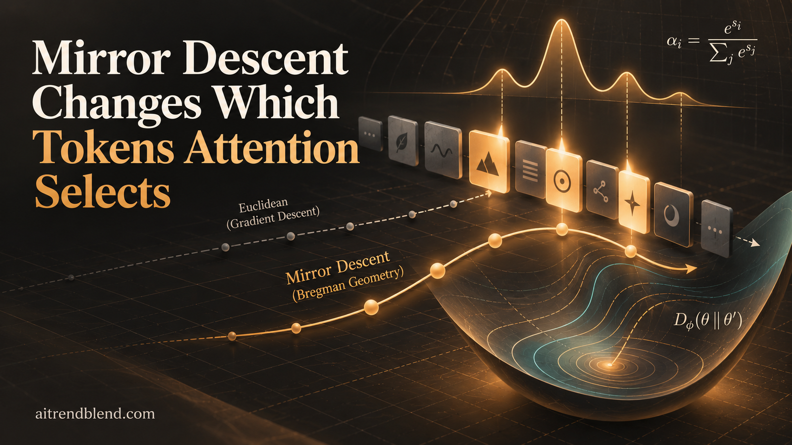
Gradient descent takes a step in the direction opposite the loss gradient using Euclidean geometry. Mirror descent replaces the Euclidean notion of movement with a geometry defined by a convex potential. Its associated Bregman divergence measures how costly a parameter change is in that geometry.
Equation 4. The potential used by the studied optimizer family and the Bregman divergence in Definition 1.
A Bregman divergence need not be symmetric. Its argument order is part of the definition, so swapping the reference direction and current direction can change the reported value. It should not be treated as an ordinary distance without qualification.
At exponent two, the potential is one half of the squared Frobenius norm and the divergence is one half of the squared Euclidean difference. The mirror descent update then reduces to gradient descent. Other exponents change both the update and its implicit preference.
The optimization step can be written in the mirror coordinates. Take the gradient of the potential, subtract a scaled loss gradient and invert the mirror map to return to the original parameters.
Equation 5. The coordinate update for the paper’s attention mirror descent algorithm.
The update is separable across coordinates, making it straightforward to implement without solving a large optimization subproblem at every step. This computational convenience is part of why the chosen potential family is useful.
The formula also shows why the exponent is an optimization choice rather than a harmless label. Near exponent one, the inverse map involves a large power. The step scale and floating point range therefore need attention. A program should expose overflow rather than silently replace the update with a different clipped rule.
What implicit bias means in this model
Implicit bias describes a preference created by the optimizer even when the objective does not explicitly ask for that preferred solution. In separable classification, gradient methods can favor particular margin directions. The paper extends that idea to token separation inside attention.
The attention matrix does not need to converge to a finite point. As its scale grows, softmax can increasingly concentrate on a selected token. Several matrices with different scales can produce similar selections, making direction the meaningful object to compare.
Theorem 8 shows norm growth under the fixed decoder assumptions, including an appropriate initialization and sufficiently small steps. The theorem gives a logarithmic lower order growth statement. Theorem 10 then shows that the normalized attention matrix approaches the normalized generalized attention SVM solution.
Equation 6. Norm growth and directional convergence from Theorems 8 and 10, conditional on their hypotheses.
A rising parameter norm is not by itself evidence that training has failed. It can coexist with a stable normalized direction and concentrated attention. But the theorem is not permission to ignore numerical overflow or to assume every growing matrix is moving toward the desired separator.
Track the direction as well as the norm. The proved limit concerns the normalized attention matrix, while the matrix itself can diverge in magnitude.
The initialization condition limits the convergence claim
The fixed decoder theorem is local. The initial attention matrix must lie inside a specified region near the target margin direction and have a sufficiently large norm. This region is defined through directional Bregman divergence and a norm threshold.
The result therefore does not say that every small random initialization reaches a globally optimal token choice. A model can have multiple locally preferred choices, and the theorem follows a trajectory starting in an appropriate region associated with one of them.
The loss assumption is also specific. It requires a strictly decreasing differentiable loss with bounded, Lipschitz derivative on closed intervals. The source lists exponential, linear decreasing and logistic losses as examples. The reference code uses logistic loss.
The step must be sufficiently small in the sense discussed in Remark 9. The potential minus the scaled loss must remain convex along the relevant trajectory. This is a condition on the analyzed path, not a universal numerical learning rate supplied for every model.
A useful distinction appears in Theorem 6. That theorem follows a regularization path of constrained optimum solutions as the permitted norm increases. It concerns globally optimal token indices and does not have the same initialization requirement as the iterative local theorem.
Following constrained optimizers is different from proving that a training algorithm finds them. Keeping those statements separate prevents a global regularization path result from becoming an unsupported promise about arbitrary gradient descent runs.
The rate is for direction, not test accuracy
Theorem 11 gives rates for the Bregman divergence between the normalized reference matrix and the normalized training iterate. These are inverse logarithmic rates in the iteration count, with different expressions for the exponent regimes.
Equation 7. The directional rate in Theorem 11.
The authors compare these rates with gradient descent in simpler linear classification settings and with earlier attention analysis that uses different assumptions. Their rate is slower than the polynomial rate they discuss from Vasudeva and colleagues, but does not require that work’s near orthogonality condition on tokens.
This is an assumption tradeoff. It is not evidence that the new optimizer reaches higher benchmark accuracy more slowly or quickly by exactly the theorem’s factor. Directional convergence, empirical loss and held out accuracy are different measurements.
The exponent regimes also should not be used as a shortcut to pick the best practical optimizer. Constants, initialization, numerical scaling and the task all matter. A better asymptotic expression for one theoretical object does not establish a better finite training run.
“our rate is logarithmic and slower”Julistiono and colleagues, Section 1.1, comparing their rate with earlier attention analysis under different assumptions
Joint training introduces a second margin problem
Once the decoder is trainable, the attention features and the classifier change together. The paper gives a joint mirror update for the attention matrix and decoder, along with a label margin SVM defined on the selected token features.
Equation 8. The decoder margin problem in Section 3.2.
The attention margin and label margin solve different tasks. The first puts a selected token above its sequence competitors. The second separates the chosen token features by class. A joint explanation has to account for both.
The strongest stated joint theorem, Theorem 31 in Appendix F, is about a regularization path with separate norm constraints. It uses an additional geometric assumption linking reduced attention on the selected token to a loss of label margin. It also couples the allowed decoder radius exponentially to the allowed attention radius.
The synthetic joint training trajectories resemble the predicted margin directions. That is useful empirical evidence, but it does not turn the regularization path theorem into a general guarantee for the joint iterative algorithm. The article keeps the theorem and simulation interpretations separate.
This distinction is especially relevant when moving to practical transformers, where the decoder, embeddings and multiple layers all change. The authors study that broader behavior experimentally rather than proving the full deep architecture version of the local single layer theorem.
Synthetic paths support the geometric interpretation
The fixed decoder synthetic experiment uses six examples, eight tokens per example and ten dimensions per token. Token vectors and comparison vectors are sampled from the unit sphere, and binary labels are randomly assigned. The experiment compares several optimizer exponents and their corresponding attention SVM directions.
The paper repeats the experiment one hundred times and reports average directional Bregman divergence with standard deviation shading. Its figures show that an optimizer path approaches the SVM direction associated with its own exponent, rather than generally approaching the directions for other exponents.
Appendix G.2 also records choices that differ from the exact constant step theory. The experiment starts near the origin and normalizes gradients to accelerate convergence. Training horizons differ across the exponent settings. These are disclosed experimental choices, not a demonstration that the initialization hypotheses can be discarded.
The chosen token indices used in the numerical SVM comparison are derived from the trained attention probabilities. That supports a comparison to the direction associated with the learned selection. It is not the same as verifying a prespecified semantic ground truth token for every random example.
Our discussion of batch size and feature learning offers related context. Optimization choices can alter which representation is selected, even when several choices fit the training objective.
The sentiment results favor a geometry close to exponent one
The practical language experiment trains transformer classifiers on the Stanford Large Movie Review Dataset. Model sizes three, four and six indicate matching numbers of encoder blocks and attention heads per block. These are deeper models than the mathematical single layer abstraction.
| Mirror potential exponent | Three blocks and heads | Four blocks and heads | Six blocks and heads |
|---|---|---|---|
| 1.1 | 83.47 ± 0.09% | 83.36 ± 0.13% | 83.65 ± 0.13% |
| 2, equivalent to GD | 81.66 ± 0.09% | 81.05 ± 0.17% | 82.22 ± 0.13% |
| 3 | 82.57 ± 0.09% | 82.40 ± 0.12% | 81.97 ± 0.10% |
The exponent 1.1 model has the highest displayed accuracy in each size. Relative to gradient descent, the mean differences are 1.81, 2.31 and 1.43 percentage points. These are arithmetic differences from the reported table, not relative percentage improvements.
The table supplies uncertainty terms, which are reproduced as printed. The accompanying text inspected here does not identify them as confidence intervals or specify their calculation clearly enough to relabel them. They should not be used to invent a significance claim.
Appendix G.4 gives a vocabulary of 30,522, an embedding dimension of 384 and a maximum token length of 512, with trainable token and position embeddings. The described model applies dropout at rate 0.2. These details help locate the experiment’s scale without implying that it fine tunes a pretrained language model.
The token examples are informative but modest evidence
The researchers also inspect attention on simple reviews generated by GPT-4o and choose pivotal tokens with that model. Figure 8 displays five examples. Its caption reports better pivotal token selection for the exponent 1.1 model in three of those five examples.
The full appendix result is more useful than that small illustration. Figure 14 reports forty sentences. Mirror descent gives strictly more attention to the designated token in twenty two cases, gradient descent wins in sixteen and two are tied.
This is a narrow comparison on generated sentences with machine designated tokens. It does not establish human validated explanations, robustness to negation or sarcasm, or a causal relationship between the highlighted token and the prediction.
Attention concentration can be a useful diagnostic. To demonstrate causal importance, one would need a separate intervention or perturbation evaluation. That is our suggested follow up, not a test reported by this paper.
The attention maps support a limited token selection comparison. They do not establish that a sharper attention map is automatically a more faithful explanation.
Vision results show comparable accuracy and different weights
The vision experiment compares four mirror descent exponents and Adam on a vision transformer. The described architecture uses patches of size four, token dimension 512, six attention blocks and eight heads per block, with dropout at rate 0.1.
Figure 10 and the accompanying text report approximately 82% test accuracy across the methods on CIFAR-10 and broadly around 55% on CIFAR-100. The article uses those approximate values rather than extracting invented exact endpoints from the plot.
The fair interpretation is competitive accuracy in the reported architecture and training setup. The evidence does not show a universal accuracy advantage over Adam, and it does not establish leadership across all configurations of these benchmarks.
The learned weights show a different pattern. The paper’s histograms suggest more concentration near zero for mirror potentials closer to exponent one. In the sentiment comparison, Figure 9 counts attention matrix entries with magnitude at least 0.06.
| Parameter family | Exponent 1.1 | Exponent 2 |
|---|---|---|
| Key weights | 18,206 | 27,224 |
| Query weights | 13,964 | 14,654 |
| Value weights | 7,643 | 10,127 |
These are threshold counts, not a measurement of exact zeros or a completed compressed model. They suggest a possible pruning opportunity. Demonstrating deployment savings would require actually pruning the weights and measuring predictive behavior, memory and runtime afterward.
The distinction connects with our article on pruning and generalization. A favorable distribution of weight magnitudes is a starting point for a compression experiment, rather than the result of one.
Runtime evidence is more useful than operation counts alone
Appendix G.1 compares the coordinate operations needed for an update when the loss gradient is already available. The source counts two operations per parameter for gradient descent, ten for mirror descent and fourteen for Adam under its accounting convention.
All scale linearly in the number of parameters, but an operation count is not a direct wall clock measurement. Powers, signs, memory traffic and fused kernels can have different costs. Gradient computation and attention computation are also outside that isolated accounting.
Appendix G.7 provides an actual training time comparison. Figure 17 follows two thousand epochs and reports approximately twenty nine hours per optimizer on CIFAR-10 and twenty five hours on CIFAR-100, with small differences across the five methods.
Those measurements support little slowdown in that setup. They do not show that mirror descent is universally faster than Adam or that the same costs hold on every accelerator. The experiments were run with an Intel i7 processor and a single V100 GPU, as described in the appendix.
How to test the method without overstating the theorem
Begin with the exact coordinate mirror update on a small attention model. Verify that exponent two gives the same update as gradient descent. Then check loss, attention probabilities, parameter norm and normalized direction as separate diagnostics.
The reference listing below includes a numerical attention SVM solver. It uses an equivalent power objective and linear token margin constraints, checking the solver’s status and returned feasibility. This supplies a comparison direction for an educational example, rather than an exact mathematical certificate.
The fixed decoder and joint decoder modes are explicit. Optional gradient normalization is also explicit and disabled by default. That prevents an acceleration choice from quietly changing the algorithm used to illustrate the constant step result.
For practical transformer comparisons, match preprocessing, architecture, initialization and training budget. Tune each optimizer’s step scale fairly rather than assuming a shared numerical learning rate is a shared effective step. Report accuracy and token diagnostics separately.
Our article on biased gradients and generalization provides another reminder that modifying an update changes the assumptions behind a proof. The authors’ experimental repository is the appropriate starting point for reproducing their real data results.
What the paper leaves open
The main proof uses a single head, one layer and, for the central iterative result, a fixed decoder. The real data experiments use broader architectures. They show that the idea is worth investigating there, but do not establish the same directional theorem for every layer of a deep transformer.
The initialization and feasibility assumptions are substantial. Finding a desirable token collection, reaching its local region and understanding the behavior of arbitrary initializations remain different questions from the conditional convergence result.
The joint regularization path requires an additional geometric margin condition and a specific relation between parameter radii. It should not be replaced by a broad statement that joint mirror descent always learns two maximum margin solutions.
Generalization evidence is empirical. The paper’s reported sentiment advantage does not establish the same benefit on unseen tasks, domains or model scales. The vision results themselves make the point that accuracy gains can be task dependent.
The interpretability and compression implications are promising but less established than the update rule and the directional analysis. Generated token examples and weight histograms cannot substitute for intervention tests or measurements of a pruned deployment.
Optimizer geometry becomes part of the attention story
The central achievement is a generalized margin characterization for mirror descent in a simplified attention model. It shows that the optimizer’s geometry can select a particular token separating direction even when the objective contains no explicit margin regularizer.
The conceptual change is to ask which solution the update favors, rather than only whether the training loss decreases. For attention, that preference concerns the competition between tokens within a sequence as well as the classifier’s separation of labels.
The experiments make the idea useful beyond the theorem. Sentiment models show a reported accuracy advantage for an exponent near one, while vision models show similar accuracy and different weight distributions. Together they support testing geometry as a design choice without promising a universal win.
The limitations preserve the result’s meaning. Directional convergence is local, joint path analysis is not a global iterative guarantee, and attention concentration is not automatically explanation fidelity. The additional deployment questions need their own measurements.
Future work can extend the theory to richer architectures and test token selection with stronger evaluations. Practitioners can already use a simpler discipline. Keep optimizer geometry, prediction quality, parameter concentration and explanation claims as separate quantities that can agree or disagree.
An attention model learns where to look. Its optimizer helps determine the geometry of that choice.
Complete PyTorch reference implementation
The listing implements the separable mirror update, the paper’s single head attention model, logistic loss, fixed and joint decoder training, evaluation, entrywise norm normalization and directional Bregman divergence. It also includes numerical attention and decoder margin solvers plus a runnable smoke test on the paper’s small example structure.
This is editorial code, not a reproduction of the multihead sentiment or vision experiments. It trains the combined attention matrix directly, with no separate key and query factorization, padding or pretrained embedding model. The selected token indices in the artificial test are explicitly supplied.
Python syntax passed. Independent numerical checks verified the mirror step’s stationarity relation at four exponents and an analytic solution for a small margin problem. PyTorch was unavailable here, so the included PyTorch smoke test was not executed. Run it with PyTorch, NumPy and SciPy before extending the example.
"""Editorial reference for Julistiono et al., JMLR 27(36), 2026.
Requires PyTorch, NumPy, SciPy. CPU float64 educational attention model.
Exact coordinate mirror update; optional normalized gradients are disclosed.
Includes fixed/joint head training and numerical attention/class SVM comparisons.
No real-data transformer reproduction or proof certification is implied.
"""
import math
import numpy as np
import torch
from torch import nn
from torch.nn import functional as F
from torch.optim import Optimizer
from scipy.optimize import linprog, minimize


def mirror_map(w, p):
    return w.sign() * w.abs().pow(p - 1)


def inverse_mirror(q, p):
    return q.sign() * q.abs().pow(1 / (p - 1))


class LpMirrorDescent(Optimizer):
    def __init__(self, params, lr=0.1, p=2., normalize_gradient=False):
        if not math.isfinite(p) or p <= 1 or not math.isfinite(lr) or lr <= 0:
            raise ValueError('Finite p>1 and positive learning rate required')
        super().__init__(params, dict(lr=lr, p=p, normalize_gradient=normalize_gradient))

    @torch.no_grad()
    def step(self, closure=None):
        loss = None
        if closure is not None:
            with torch.enable_grad(): loss = closure()
        for group in self.param_groups:
            for w in group['params']:
                if w.grad is None: continue
                if w.grad.is_sparse: raise ValueError('Dense gradients required')
                grad = w.grad
                if not torch.isfinite(grad).all(): raise FloatingPointError('Nonfinite gradient')
                if group['normalize_gradient']:
                    # Appendix G.2 uses normalized gradients for its synthetic paths.
                    # This changes the step scaling from the constant-step theorem.
                    size = grad.norm()
                    grad = grad / size if size.item() > 0 else grad
                dual = mirror_map(w, group['p']) - group['lr'] * grad
                updated = inverse_mirror(dual, group['p'])
                if not torch.isfinite(updated).all():
                    raise FloatingPointError('Mirror update overflow; reduce step size')
                w.copy_(updated)
        return loss


class SoftmaxAttentionClassifier(nn.Module):
    def __init__(self, d, decoder=None, train_decoder=False, seed=42):
        super().__init__()
        gen = torch.Generator().manual_seed(seed)
        self.W = nn.Parameter(torch.zeros(d, d, dtype=torch.float64))
        v = torch.randn(d, generator=gen, dtype=torch.float64)
        v = v / v.norm()
        if decoder is not None: v = torch.as_tensor(decoder, dtype=torch.float64).clone()
        if train_decoder: self.v = nn.Parameter(v)
        else: self.register_buffer('v', v)

    def forward(self, x, z, return_attention=False):
        # x: [n,T,d], z: [n,d], W: [d,d]. No sqrt(d) rescaling in Eq. (2).
        if x.ndim != 3 or z.shape != (x.shape[0], x.shape[2]):
            raise ValueError('Expected x[n,T,d] and z[n,d]')
        query = z @ self.W.T
        logits = torch.einsum('ntd,nd->nt', x, query)
        probability = logits.softmax(dim=1)
        feature = torch.einsum('nt,ntd->nd', probability, x)
        score = feature @ self.v
        return (score, probability) if return_attention else score


def logistic_loss(score, y):
    return F.softplus(-y * score).mean()


def validate_labels(y):
    if not torch.all((y == -1) | (y == 1)):
        raise ValueError('Expected binary labels -1,+1')


def lp_normalized(w, p):
    size = w.flatten().norm(p=p)
    return w / size if size.item() > 0 else torch.zeros_like(w)


def bregman(reference, current, p):
    # D_psi(reference,current), the orientation used in Theorem 11.
    potential_a = reference.abs().pow(p).sum() / p
    potential_b = current.abs().pow(p).sum() / p
    return potential_a - potential_b - (mirror_map(current, p) * (reference-current)).sum()


def train(model, x, y, z, steps=200, p=2., lr_w=0.1, lr_v=0.1, normalize_gradient=False):
    validate_labels(y)
    groups = [{'params':[model.W], 'lr':lr_w}]
    if isinstance(model.v, nn.Parameter): groups.append({'params':[model.v], 'lr':lr_v})
    optimizer = LpMirrorDescent(groups, p=p, normalize_gradient=normalize_gradient)
    history=[]
    for _ in range(steps):
        optimizer.zero_grad(set_to_none=True)
        score, probability = model(x,z,True)
        loss=logistic_loss(score,y)
        loss.backward()
        history.append({'loss':loss.item(), 'W_norm':model.W.detach().flatten().norm(p=p).item(),
                        'mean_max_attention':probability.detach().max(dim=1).values.mean().item()})
        optimizer.step()
    return history


@torch.no_grad()
def evaluate(model,x,y,z,alpha=None, threshold=0.06):
    validate_labels(y)
    score,prob=model(x,z,True)
    predicted=torch.where(score>=0,1.,-1.)
    report={'loss':logistic_loss(score,y).item(), 'accuracy':(predicted==y).double().mean().item(),
            'mean_max_attention':prob.max(dim=1).values.mean().item(),
            'attention_entropy':(-(prob*prob.clamp_min(1e-300).log()).sum(1)).mean().item(),
            'weights_above_threshold':(model.W.abs()>=threshold).sum().item()}
    if alpha is not None:
        report['chosen_token_probability']=prob.gather(1,alpha[:,None]).mean().item()
    return report


def solve_lp_margin(A,p):
    """Minimize sum |w|^p /p under A w >= 1 using a numerical convex solve.
    SLSQP status and feasibility are checked; not an exact proof certificate.
    """
    A=np.asarray(A,dtype=float)
    feasible=linprog(np.zeros(A.shape[1]),A_ub=-A,b_ub=-np.ones(A.shape[0]),
                     bounds=[(None,None)]*A.shape[1],method='highs')
    if not feasible.success: raise ValueError('Margin constraints infeasible')
    objective=lambda w:(np.abs(w)**p).sum()/p
    derivative=lambda w:np.sign(w)*np.abs(w)**(p-1)
    result=minimize(objective,feasible.x,jac=derivative,method='SLSQP',
                    constraints=[{'type':'ineq','fun':lambda w:A@w-1,'jac':lambda w:A}],
                    options={'ftol':1e-10,'maxiter':5000})
    if not result.success or (A@result.x).min()<1-1e-6:
        raise RuntimeError('Numerical margin solve failed validation')
    return torch.tensor(result.x,dtype=torch.float64)


def attention_svm(x,z,alpha,p):
    n,T,d=x.shape;rows=[]
    for i in range(n):
        for t in range(T):
            if t!=alpha[i].item(): rows.append(torch.outer(x[i,alpha[i]]-x[i,t],z[i]).flatten())
    return solve_lp_margin(torch.stack(rows).detach().numpy(),p).reshape(d,d)


def decoder_svm(x,y,alpha,p):
    chosen=x[torch.arange(len(x)),alpha]
    return solve_lp_margin((y[:,None]*chosen).detach().numpy(),p)


def synthetic_data(n=6,T=8,d=10,seed=7):
    gen=torch.Generator().manual_seed(seed)
    x=torch.randn(n,T,d,generator=gen,dtype=torch.float64);x=x/x.norm(dim=-1,keepdim=True)
    z=torch.randn(n,d,generator=gen,dtype=torch.float64);z=z/z.norm(dim=-1,keepdim=True)
    y=(2*torch.randint(0,2,(n,),generator=gen)-1).double()
    return x,y,z


def example_one():
    x=torch.tensor([[[5.,0.],[0.,1.]],[[-5.,0.],[0.,-1.]]],dtype=torch.float64)
    return x,torch.tensor([1.,-1.],dtype=torch.float64),x[:,0].clone()


def smoke_test():
    # Exact p=2 update equals GD for one step, including signed and zero coordinates.
    w=nn.Parameter(torch.tensor([0.,-0.2,0.4],dtype=torch.float64))
    grad=torch.tensor([0.1,-0.3,0.2],dtype=torch.float64);initial=w.detach().clone();w.grad=grad
    LpMirrorDescent([w],lr=0.05,p=2).step()
    assert torch.allclose(w,initial-0.05*grad,atol=1e-14)
    for p in [1.1,1.75,2.,3.]:
        values=torch.tensor([-.3,0.,.8],dtype=torch.float64)
        assert torch.allclose(inverse_mirror(mirror_map(values,p),p),values,atol=1e-12)
    x,y,z=example_one();alpha=torch.zeros(2,dtype=torch.long)
    for p in [1.75,2.,3.]:
        model=SoftmaxAttentionClassifier(2,decoder=[1.,0.])
        history=train(model,x,y,z,steps=80,p=p,lr_w=0.01)
        assert history[-1]['loss']<history[0]['loss']
        assert torch.isfinite(model.W).all()
        reference=attention_svm(x,z,alpha,p)
        distance=bregman(lp_normalized(reference,p),lp_normalized(model.W.detach(),p),p)
        assert distance.item()>=-1e-10
        print(p,evaluate(model,x,y,z,alpha), 'directional Bregman:',distance.item())
    joint=SoftmaxAttentionClassifier(2,decoder=[1.,0.],train_decoder=True)
    train(joint,x,y,z,steps=20,p=2.,lr_w=.01,lr_v=.01)
    assert torch.isfinite(joint.v).all()
    print('Smoke checks passed; no asymptotic theorem or real benchmark was reproduced.')


if __name__=='__main__':
    smoke_test()
Frequently asked questions
How is mirror descent different from gradient descent?
It updates in coordinates defined by a convex potential and uses the associated Bregman geometry. For the squared Euclidean potential, its update reduces to gradient descent.
What does the attention SVM separate?
It separates a chosen token from the other tokens within each example using attention logits. The decoder SVM instead separates selected token features by label.
Does the convergence theorem cover every initialization?
No. The central fixed decoder theorem requires feasibility, locally optimal token indices, an appropriate initial direction and norm, and sufficiently small steps.
Does the joint theorem guarantee arbitrary joint training?
No. The stated joint theorem concerns constrained optimum solutions along a regularization path with additional geometric assumptions. The joint iterative examples provide supporting simulations.
Did mirror descent outperform Adam on the image benchmarks?
The reported vision experiments reach broadly similar accuracy across the compared optimizers. Weight distributions differ, but the paper does not establish a universal accuracy advantage over Adam.
Has the included code reproduced the published experiments?
No. It is an editorial single head reference implementation. Syntax and independent numerical mirror and margin checks passed, but its PyTorch smoke test was not run here.
Read the analysis and reproduce the experiments
The paper supplies the complete assumptions and proofs. The authors’ repository contains synthetic and real data experiment code.
Read the JMLR paperAuthors’ experimental codeJulistiono, A. K., Ataee Tarzanagh, D., and Azizan, N. (2026). Optimizing Attention with Mirror Descent, Generalized Max Margin Token Selection. Journal of Machine Learning Research, 27(36), pages 1 to 61. Title punctuation simplified. Official publication record.
This analysis is based on the published paper and an independent evaluation of its claims.