
Key points
- The authors release DSCA, a publicly available dataset of 224 digital subtraction angiography sequences from 58 patients, with pixel level annotations distinguishing main artery trunks from bifurcated vessels.
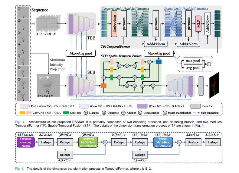
- DSANet processes the full sequence through a dedicated temporal branch and a minimum intensity projection image through a spatial branch, rather than segmenting a single frame the way most prior methods do.
- A module called TemporalFormer applies self attention across time and then across space to capture how vessels fill with contrast dye across frames.
- A Spatio-Temporal Fusion module combines the two branches, and the paper reports this combination suppresses false positives from residual skull structures that other methods mistake for vessels.
- DSANet reached a Dice of 0.9033 on the main artery trunk and outperformed ten comparison methods, including nnU-Net and several transformer based segmentation architectures, across nearly every metric reported.
- Ablation experiments show each added component, the temporal branch, the TemporalFormer, and the fusion module, contributes a measurable improvement, most visibly on the main artery trunk and on vessel connectivity.
Why a single frame is the wrong unit of analysis
Cerebrovascular diseases, stroke, moyamoya disease, and cerebral aneurysms among them, remain a major cause of death and disability, and diagnosing them accurately depends on understanding the geometry of the cerebral arteries. Digital subtraction angiography, often shortened to DSA, is the technique clinicians turn to when other imaging methods such as CT angiography or MR angiography cannot resolve a case with enough confidence, because DSA captures both the fine spatial detail of the vessels and the temporal dynamics of blood flow through them.
That temporal dimension is exactly what most automated segmentation research has ignored. A DSA sequence typically runs to somewhere between 5 and 22 arterial phase frames, and each individual frame only shows a fraction of the contrast agent as it moves through the vasculature. Training a network on a single extracted frame, which is how the authors describe the majority of prior DSA segmentation work, means the network never sees the full picture of how the vessel tree fills, and the paper reports this leads to unstable segmentation of the smallest, hardest to see vessels.
Inside the DSCA dataset
DSCA was collected from intraoperative and postoperative DSA imaging at the First Affiliated Hospital of Zhengzhou University between January 2022 and July 2023, with patient identifiers removed and collection approved by the hospital’s ethics committee. The dataset covers 58 patients, 28 male and 30 female, ranging from 9 to 81 years old, and totals 224 DSA sequences comprising 1,792 images captured across three different arteries, the internal carotid artery, the external carotid artery, and the vertebral artery. The sequences were captured on a mix of Siemens, Philips, and Shimadzu imaging systems, which the authors report as a strength, since it means a model trained on DSCA has seen some of the natural variation that shows up across different hospital equipment rather than a single vendor’s output.
The annotation protocol is worth walking through because it is where a lot of the paper’s clinical care shows up. Five clinicians with more than five years of experience each annotated a portion of the 224 MinIP images once, using a tool called ITK-SNAP. Disputed annotations went to a senior neurosurgeon, and if two senior reviewers disagreed, they worked together to reach a consensus rather than a single reviewer breaking the tie. Vessels in the internal carotid and vertebral artery sequences were labeled into three categories, background, bifurcated vessels, and the main artery trunk, with the boundary between trunk and branch defined by established anatomical segments, the C7 segment for the internal carotid artery and the V4 segment for the vertebral artery. External carotid artery sequences, which lack a single dominant trunk, were only labeled as background or bifurcated vessel.
| Dataset | Samples | Type | Publicly available |
|---|---|---|---|
| Meng et al. | 30 | Single frame | No |
| Vepa et al. | 128 | Single frame | No |
| DIAS | 120 | Sequence | Yes |
| DSCA (this paper) | 224 | Sequence, multiple resolutions | Yes |
Adapted from Table II in the paper. DSCA is compared against five prior single frame datasets and DIAS, the only other publicly released DSA sequence dataset the authors identify.
That comparison against DIAS matters. Prior to this paper, DIAS was the only other public sequence level DSA dataset, and it contains 120 labeled and unlabeled samples combined without detailed pathological descriptions. DSCA is roughly double the labeled sample count, spans multiple resolutions rather than one fixed size, and includes explicit trunk versus branch labeling that DIAS does not, which the authors argue matters clinically because separating the main trunk from bifurcated branches supports tasks such as automated stenosis measurement and vessel labeling that a plain vessel or no vessel mask cannot support on its own.
How DSANet actually processes a sequence
DSANet is built around two parallel encoding branches that share the same five layer convolutional structure but never share weights. The spatial encoding branch takes the single MinIP image as input. The temporal encoding branch takes the full resampled sequence, all sequences are resampled to a fixed 8 frames since the authors found that was close to the natural distribution of arterial phase frame counts across the dataset and that resampling to significantly more or fewer frames hurt performance in their ablation experiments. Skip connections from each of the first four layers of both branches are combined and passed to a shared decoder, so spatial and temporal information gets threaded through the network at multiple resolutions rather than only at the bottleneck.
TemporalFormer, treating each frame as a token
The feature that separates DSANet’s temporal branch from a generic 3D convolutional network is TemporalFormer. After the temporal branch extracts features from each frame, TemporalFormer treats every frame’s feature map as a single token in a sequence and runs self attention across those tokens, which lets the network learn correlations between frames that are far apart in time, not just adjacent ones. A learnable position encoding is added to each frame’s token before this attention step so the network retains a sense of frame order.
Eq. 1 and Eq. 2 in the paper. The same self attention formulation runs twice per TemporalFormer layer, once across the temporal axis to relate frames to each other and once across the spatial axis to relate pixel locations within a frame.
After the temporal attention step, the same self attention operation is applied a second time, now across spatial locations within each frame rather than across frames, and the two outputs are combined with residual connections before a small multilayer perceptron refines the result. The paper stacks four of these TemporalFormer layers, then downsamples across the time dimension to collapse the sequence back down to a single feature map that carries the accumulated temporal context forward into the fusion stage.
Spatio-Temporal Fusion, letting the two branches correct each other
Having two separate feature maps, one spatial and one temporal, is not automatically useful unless they get combined well. The Spatio-Temporal Fusion module, STF for short, pools both feature maps down to save computation, projects them through a shared convolutional block, and computes a cross attention style weighting between the two using the same query, key, value pattern as TemporalFormer, but this time relating the spatial and temporal features to each other rather than relating frames or pixels within a single branch.
The paper’s stated motivation for this design is specific and testable, that the dynamic changes of vessels across frames and the structural invariance of the skull across frames give the network two independent signals it can cross check, and the paper’s qualitative results back this up directly. Skull fragments with strong contrast are mistaken for vessels by several comparison methods, but DSANet’s error maps show it successfully suppressing those false positives in cases where the temporal signal would have shown the false structure was not actually changing the way a real vessel does across the sequence.
How well it actually performs
The authors compare DSANet against ten methods spanning DSA specific architectures and general purpose medical segmentation networks, including UNet, CE-Net, AttentionUNet, SwinUNet, TransUNet, H2Former, and nnU-Net, all retrained on DSCA under the same five fold cross validation protocol for a fair comparison.
| Method | Dice, main trunk | Dice, bifurcated vessel | clDice, whole vessel |
|---|---|---|---|
| UNet | 77.68 percent | 82.34 percent | 84.34 percent |
| TransUNet | 78.41 percent | 83.34 percent | 84.68 percent |
| H2Former | 88.34 percent | 84.06 percent | 82.30 percent |
| nnU-Net | 89.69 percent | 86.22 percent | 87.54 percent |
| DSANet, ours | 92.26 percent | 87.32 percent | 88.58 percent |
DSANet reached the best score on every metric reported for both the main artery trunk and bifurcated vessel classes. The gap is largest on the main trunk, where DSANet surpassed H2Former, the strongest comparison method on that class, by 3.92 percentage points of Dice, a difference the authors report as statistically significant. On bifurcated vessels, which occupy a smaller share of the image and are consequently harder to move the needle on, the improvement over nnU-Net was a more modest 1.11 percentage points of Dice, still statistically significant but a reminder that thin, low contrast structures remain the harder half of this problem regardless of architecture.
What the ablation study actually isolates
The ablation experiments are where this paper earns its architectural claims rather than just asserting them. Starting from nnU-Net as a baseline, the authors added the temporal encoding branch alone, then TemporalFormer on top of that, then the STF module on top of that, and measured each addition’s effect separately.
Adding the temporal branch alone produced more than a one percentage point increase across JAC, Dice, sensitivity, precision, and AUC specifically on the main artery trunk, which the authors attribute to the branch capturing dynamic flow information a single MinIP image cannot show. Adding TemporalFormer on top of the temporal branch produced a further improvement concentrated even more heavily on the main trunk than on bifurcated vessels, with sensitivity for the trunk reaching what the paper reports as its best value across the whole ablation series, 91.86 percent. Adding the STF module on top of both prior components produced the largest precision gains of the three additions, 4.95 percentage points over the baseline on the main trunk, which lines up with the qualitative finding that STF is what actually suppresses the residual skull false positives, precision being exactly the metric that punishes false positive predictions most directly.
One honest wrinkle the authors report themselves, after adding both TemporalFormer and STF together, the combined model’s sensitivity was slightly lower than versions with only one of the two components added, even though every other metric improved. Their interpretation is that stacking both components increases the model’s tendency to flag borderline false positives in the background, which the STF module was specifically built to suppress, so the combination trades a small amount of recall for a larger gain in precision and overall segmentation quality, a genuine tradeoff rather than a strictly dominant improvement on every axis.
Where the model still struggles, and what the authors tested to find out
The paper runs several additional experiments specifically aimed at probing its own limits rather than only showcasing wins. Running the TemporalFormer’s temporal and spatial attention steps in parallel instead of one after another performed worse, particularly on distinguishing the main trunk from bifurcated vessels, which the authors interpret as evidence that combining the two attention signals directly, without processing them in sequence, creates interference between the temporal and spatial representations. Swapping the standard Dice loss for a topology focused clDice loss during training also underperformed, with the authors noting that clDice’s emphasis on vessel centerlines can come at the expense of accuracy on larger vessel structures. A variable length sequence input, rather than the fixed 8 frame resampling used everywhere else in the paper, performed better than a naively fixed length alternative but still fell short of the original resampled approach, which restricts batch size to 1 and is harder to train.
Trying the core modules yourself
The two components that make DSANet different from a standard 2D segmentation network are TemporalFormer, which runs attention across frames and then across space, and the Spatio-Temporal Fusion module, which merges the resulting temporal feature with the spatial MinIP feature. Implementing both directly, with realistic tensor shapes for a batch of resampled 8 frame sequences, shows exactly how the reshaping described in the paper’s Fig. 4 turns a 5 dimensional sequence tensor into something a standard attention layer can consume.
"""
DSANet core modules: TemporalFormer (TF) and Spatio-Temporal Fusion (STF)
Implementation of the components from Zhang et al. (2025)
DSCA, A Digital Subtraction Angiography Sequence Dataset and
Spatio-Temporal Model for Cerebral Artery Segmentation
IEEE Transactions on Medical Imaging, vol. 44, no. 6

Educational note, this is not clinical software and is not validated
for diagnostic use.
"""

import torch
import torch.nn as nn
import torch.nn.functional as F


# 1. TemporalFormer, Eq. 1 and Eq. 2, dimension flow shown in Fig. 4.

class TemporalFormerLayer(nn.Module):
    def __init__(self, channels, num_heads=8):
        super().__init__()
        self.temporal_attn = nn.MultiheadAttention(channels, num_heads, batch_first=True)
        self.spatial_attn = nn.MultiheadAttention(channels, num_heads, batch_first=True)
        self.norm1 = nn.LayerNorm(channels)
        self.norm2 = nn.LayerNorm(channels)
        self.mlp = nn.Sequential(
            nn.Linear(channels, channels * 2),
            nn.GELU(),
            nn.Linear(channels * 2, channels),
        )

    def forward(self, x, b, t, h, w):
        # x arrives as [B, T, H*W, C] so temporal attention runs per pixel
        c = x.shape[-1]

        # Temporal self attention, Eq. 1 and Eq. 2, over the T axis
        x_temporal = x.permute(0, 2, 1, 3).reshape(b * h * w, t, c)
        attn_out, _ = self.temporal_attn(x_temporal, x_temporal, x_temporal)
        x_temporal = x_temporal + attn_out
        x_temporal = x_temporal.reshape(b, h * w, t, c).permute(0, 2, 1, 3)

        # Spatial self attention over the hw axis, same formulation
        x_spatial = x_temporal.reshape(b * t, h * w, c)
        attn_out, _ = self.spatial_attn(x_spatial, x_spatial, x_spatial)
        x_spatial = x_spatial + attn_out
        x_spatial = self.norm1(x_spatial)

        out = x_spatial + self.mlp(x_spatial)
        out = self.norm2(out)
        return out.reshape(b, t, h * w, c)


class TemporalFormer(nn.Module):
    def __init__(self, channels, num_layers=4, num_heads=8, max_frames=16):
        super().__init__()
        self.pos_embed = nn.Parameter(torch.zeros(max_frames, channels))
        nn.init.trunc_normal_(self.pos_embed, std=0.02)
        self.layers = nn.ModuleList(
            [TemporalFormerLayer(channels, num_heads) for _ in range(num_layers)]
        )

    def forward(self, f_s):
        # f_s: [B, T, C, H, W] features from the Temporal Encoding Branch
        b, t, c, h, w = f_s.shape
        x = f_s.permute(0, 1, 3, 4, 2).reshape(b, t, h * w, c)
        x = x + self.pos_embed[:t].reshape(1, t, 1, c)

        for layer in self.layers:
            x = layer(x, b, t, h, w)

        x = x.reshape(b, t, h, w, c).permute(0, 1, 4, 2, 3)
        return x.mean(dim=1)  # downsample the T dimension


# 2. Spatio-Temporal Fusion module, Eq. 3 and Eq. 4.

class SpatioTemporalFusion(nn.Module):
    def __init__(self, channels):
        super().__init__()
        self.shared_proj = nn.Conv2d(channels, channels, kernel_size=1)
        self.q_proj = nn.Conv2d(channels, channels, kernel_size=1)
        self.k_proj = nn.Conv2d(channels, channels, kernel_size=1)
        self.v_proj = nn.Conv2d(channels, channels, kernel_size=1)
        self.channels = channels

    def _project(self, feat):
        feat = self.shared_proj(feat)
        return self.q_proj(feat), self.k_proj(feat), self.v_proj(feat)

    def forward(self, f_m, f_s):
        b, c, h, w = f_m.shape

        # Maxpool both features to reduce resolution and noise
        f_m_pooled = F.max_pool2d(f_m, 2)
        f_s_pooled = F.max_pool2d(f_s, 2)
        hp, wp = f_m_pooled.shape[-2:]

        q_m, k_m, v_m = self._project(f_m_pooled)
        q_s, k_s, v_s = self._project(f_s_pooled)

        def flat(t):
            return t.flatten(2).transpose(1, 2)

        q_m, k_m, v_m = flat(q_m), flat(k_m), flat(v_m)
        q_s, k_s, v_s = flat(q_s), flat(k_s), flat(v_s)

        scale = self.channels ** 0.5
        alpha_m = torch.softmax((q_m @ k_m.transpose(1, 2)) / scale, dim=-1)
        alpha_s = torch.softmax((q_s @ k_s.transpose(1, 2)) / scale, dim=-1)

        # Eq. 3, the two weight matrices are summed then applied to each value
        combined = alpha_m + alpha_s
        f_m_enh = combined @ v_m
        f_s_enh = combined @ v_s

        fused = torch.cat([f_m_enh, f_s_enh], dim=-1)
        fused = fused.transpose(1, 2).reshape(b, 2 * c, hp, wp)
        fused = F.interpolate(fused, size=(h, w), mode="bilinear", align_corners=False)

        # Eq. 4, add the upsampled fused feature to the plain concatenation
        return fused + torch.cat([f_s, f_m], dim=1)


# 3. Smoke test with synthetic DSA-like sequence and MinIP features.

if __name__ == "__main__":
    torch.manual_seed(0)

    batch_size = 2
    num_frames = 8    # DSCA resamples every sequence to 8 frames
    channels = 32
    height, width = 16, 16

    f_s_seq = torch.randn(batch_size, num_frames, channels, height, width)
    f_m = torch.randn(batch_size, channels, height, width)

    tf_module = TemporalFormer(channels, num_layers=4, num_heads=4, max_frames=num_frames)
    stf_module = SpatioTemporalFusion(channels)
    tf_module.eval()
    stf_module.eval()

    with torch.no_grad():
        f_s = tf_module(f_s_seq)
        fused = stf_module(f_m, f_s)

    print(f"TEB sequence input:     {tuple(f_s_seq.shape)}")
    print(f"TemporalFormer output:  {tuple(f_s.shape)}")
    print(f"SEB MinIP input:        {tuple(f_m.shape)}")
    print(f"STF fused output:       {tuple(fused.shape)}")

    assert f_s.shape == (batch_size, channels, height, width)
    assert fused.shape == (batch_size, 2 * channels, height, width)

    seg_head = nn.Conv2d(2 * channels, 3, kernel_size=1)  # background, BV, MAT
    logits = seg_head(fused)
    print(f"Segmentation logits:    {tuple(logits.shape)}")
    assert logits.shape == (batch_size, 3, height, width)

    print("Smoke test complete. TemporalFormer and Spatio-Temporal Fusion ran end to end without error.")
Running this script confirms the full reshape chain works, an 8 frame sequence tensor goes into TemporalFormer and comes out as a single feature map with the batch and channel dimensions preserved, that feature map is fused with a separately encoded MinIP feature map through STF into a tensor with double the channel count, and a segmentation head on top produces per pixel scores across the paper’s three classes, background, bifurcated vessel, and main artery trunk.
Where this fits in the broader picture
Medical image segmentation research has generally treated architecture innovation, better skip connections, attention mechanisms, transformer blocks, as the main lever for progress, largely because the field’s benchmark datasets have mostly been single frame or single volume by construction. This paper’s contribution sits one level upstream of architecture, arguing that for an inherently dynamic imaging modality like DSA, the dataset itself needs to preserve the temporal dimension or no amount of architectural cleverness applied to a single frame can recover the information that was thrown away during data preparation. The MinIP labeling strategy is a genuinely practical answer to the annotation cost problem that a naive full sequence labeling approach would create, and it is the kind of dataset design decision that tends to get imitated once it is shown to work.
It is also worth situating this against DIAS, the other public DSA sequence dataset the authors compare against directly. DSANet outperforms VSSNet, a method specifically built for the DIAS benchmark, on JAC, Dice, and precision when both are evaluated on DSCA, though the authors are transparent that VSSNet edges out DSANet on sensitivity and AUC, meaning VSSNet tends to catch more true positives at the cost of more false positives, a genuine trade off between the two approaches rather than a clean win for either one.
Conclusion
The headline number, a Dice of 0.9033, is not really the interesting part of this paper on its own, plenty of segmentation papers report strong Dice scores. What makes this one worth attention is the two part argument underneath the number, that DSA is fundamentally a temporal imaging modality being analyzed with spatial only tools, and that the fix does not require abandoning the practical need for efficient annotation, it just requires separating what gets labeled, the MinIP image, from what the network actually learns from, the full sequence.
The ablation study earns its keep here. Rather than presenting TemporalFormer and STF as a fait accompli, the paper isolates each component’s contribution and is candid about a real tradeoff, the fully combined model gives up a small amount of sensitivity in exchange for large gains in precision and connectivity. That kind of transparency about what a design choice costs, not just what it buys, is worth more than another headline metric.
The clinical framing matters too. Separating main trunk from bifurcated vessel is not an arbitrary extra label category, the authors tie it directly to real downstream tasks, automated stenosis measurement and vessel labeling, that a plain binary vessel mask cannot support. Whether DSCA and DSANet get adopted as a standard benchmark the way DIAS has started to will depend on exactly this kind of usefulness beyond the leaderboard.
The clearest limitation is scope. This is a single hospital, 58 patient dataset, and the authors do not claim otherwise, framing DSCA as a contribution to a field that has been starved of public sequence level data rather than as a definitive benchmark. Generalization to other hospitals, other imaging vendors beyond the three represented here, and other patient populations remains an open question the paper’s own DIAS cross evaluation experiment only partially addresses.
Read the original paper
Zhang, J., Xie, Q., Mou, L., Zhang, D., Chen, D., Shan, C., Zhao, Y., Su, R., and Guo, M. DSCA, A Digital Subtraction Angiography Sequence Dataset and Spatio-Temporal Model for Cerebral Artery Segmentation. IEEE Transactions on Medical Imaging, volume 44, number 6, June 2025. DOI 10.1109/TMI.2025.3540886.
Frequently asked questions
What is digital subtraction angiography
Digital subtraction angiography, or DSA, is an imaging technique that captures a sequence of x-ray frames as contrast dye moves through blood vessels, then subtracts a baseline image to isolate the vessels from surrounding tissue. It is considered the gold standard for diagnosing cerebrovascular disease when other techniques such as CT angiography or MR angiography cannot resolve a case clearly.
What makes the DSCA dataset different from earlier DSA datasets
Most earlier DSA segmentation datasets provide only a single labeled frame per case and are not publicly released. DSCA provides 224 full sequences with pixel level annotations on a minimum intensity projection image, distinguishes main artery trunk from bifurcated vessels, spans three different arteries and multiple imaging resolutions, and is publicly available on GitHub.
How does DSANet use a whole sequence instead of one frame
DSANet has two parallel branches, one that processes the single MinIP image for spatial detail and one that processes the full 8 frame resampled sequence for temporal detail. A module called TemporalFormer applies self attention across frames and then across spatial locations, and a Spatio-Temporal Fusion module combines the two branches before the result is decoded into a segmentation map.
How accurate is DSANet
DSANet reached a Dice score of 0.9033 on the main artery trunk class and outperformed all ten comparison methods the authors tested, including nnU-Net and several transformer based segmentation architectures, across nearly every metric reported, with statistically significant improvements on the main trunk class in particular.
Is DSANet ready for clinical use
No. It is a research contribution evaluated on a single hospital dataset of 58 patients. The paper itself frames its contribution as advancing a research field that has lacked public data, not as a validated diagnostic tool, and clinical adoption would require substantially more validation across institutions, scanners, and patient populations.
What does the ablation study show about which component matters most
Adding the temporal encoding branch alone produced over a one percentage point gain on the main trunk across several metrics. Adding TemporalFormer on top improved sensitivity further, reaching 91.86 percent on the main trunk. Adding the Spatio-Temporal Fusion module on top of both produced the largest precision gains, 4.95 percentage points over the baseline, which lines up with its role in suppressing false positives from residual skull structures.