The Aggregator Everyone Dismissed Just Turned Out to Be the Best Defense Against Label Poisoning
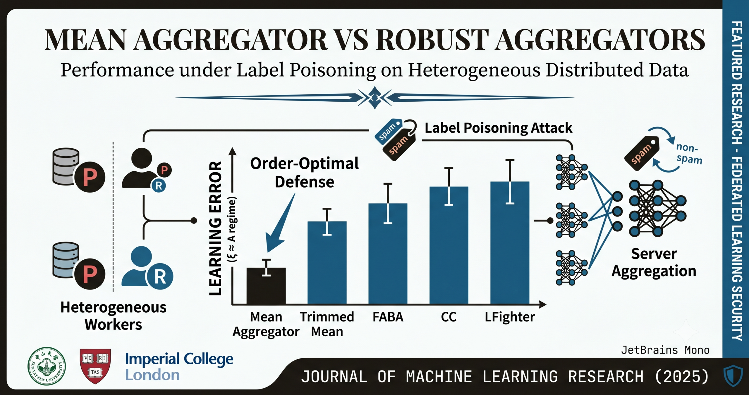
A team from Sun Yat-Sen University, Harvard, and Imperial College London has flipped the conventional wisdom of Byzantine-robust distributed learning: when attacks are confined to label poisoning and data is heterogeneous enough, the plain old mean aggregator outperforms — and matches the theoretical optimum of — every sophisticated robust aggregator on the market.
There is an old assumption in distributed machine learning that has gone mostly unchallenged for a decade: robust aggregators are better than the mean. The logic seemed airtight — if some workers send poisoned gradients, averaging everything naively amplifies the poison. So the field built trimmed means, geometric medians, centered clipping algorithms, and a growing zoo of Byzantine-tolerant methods, all designed to push out malicious contributions. Jie Peng, Weiyu Li, Stefan Vlaski, and Qing Ling just showed that this logic, while correct for worst-case attacks, breaks down completely for one of the most common real-world threats: label poisoning. Their proof, published in JMLR in 2025, is both unsettling and clarifying in equal measure.
What Label Poisoning Actually Looks Like in the Wild
To understand why the result matters, you have to think concretely about how attacks actually happen in deployed distributed systems — not in the clean theoretical models that most papers use. The Byzantine adversary model, which dominates the robustness literature, assumes that compromised workers can send anything to the server: arbitrary vectors, adversarially crafted gradients, complete nonsense. It is worst-case by design. And for that specific threat, robust aggregators do what they promise.
But consider a more realistic scenario. A large organization is running federated training of a spam detection model across thousands of user devices. A subset of those users start mislabeling emails — marking obvious spam as “not spam” because they want certain messages to get through. These users are not sophisticated attackers. They follow the protocol exactly; they just compute gradients on corrupted data. Their gradients are wrong, but they are wrong in a structured, bounded way.
That is label poisoning. The poisoned workers have corrupted labels, not corrupted algorithms. They compute their local stochastic gradients faithfully from poisoned data, update their local momentum honestly, and send the result to the server. The disturbance they introduce is bounded — you can upper-bound it in terms of the feature norms of their data. This is categorically different from Byzantine behavior, and it creates a fundamentally different mathematical structure that robust aggregators are — it turns out — poorly suited to handle.
Byzantine attacks allow arbitrary, unbounded malicious messages. Label poisoning attacks produce incorrect but bounded, structured perturbations — because the attackers still follow the algorithmic protocol, they just do so on corrupted labels. Robust aggregators were designed for the former. They pay a price in the latter that the mean aggregator does not.
Why Robust Aggregators Pay a Hidden Tax
Here is the core tension that the paper exposes. Robust aggregators — trimmed mean, FABA, centered clipping, and their cousins — work by finding a point that is close to the average of the honest workers’ gradients regardless of what the poisoned workers send. The approximation guarantee they achieve is stated in terms of a contraction constant ρ: the aggregator’s output is within ρ times the heterogeneity of the honest gradients from their true average.
The problem is that ρ can never be zero. A robust aggregator cannot tell which workers are regular and which are poisoned, so it must hedge. The smaller the fraction of poisoned workers, the smaller ρ can be — but it cannot vanish. And the non-vanishing learning error of algorithms using a ρ-robust aggregator scales as O(ρ²ξ²), where ξ is the heterogeneity of the honest workers’ local gradients.
Now think about what happens as the data becomes more heterogeneous — which is exactly the realistic federated setting, where workers often have data from completely different distributions. As ξ grows, the baseline error of robust aggregators grows quadratically with it. For trimmed mean, the contraction constant itself blows up as the fraction of poisoned workers approaches 1/2; for FABA, it blows up even faster, near 1/3. These methods were designed for attacks where the adversary can cause unbounded damage. When the damage is bounded, their conservatism becomes a liability.
The mean aggregator, by contrast, does not try to filter anything out. Its non-vanishing error under label poisoning scales as O(δ²A²), where δ is the fraction of poisoned workers and A bounds the disturbance each poisoned worker can cause. And here is the crucial insight: when data is sufficiently heterogeneous, A and ξ are in the same order. Under that condition, O(δ²A²) is both smaller than any robust aggregator’s error and matches the information-theoretic lower bound for the problem.
“The robust aggregators are too conservative for a class of weak but practical malicious attacks. The mean aggregator is not just competitive — its learning error is order-optimal regardless of the fraction of poisoned workers.” — Peng, Li, Vlaski, and Ling, JMLR (2025)
The Mathematical Setup: Distributed Stochastic Momentum
The paper works within distributed stochastic momentum, a framework that generalizes both distributed gradient descent and distributed stochastic gradient descent. At each iteration, the server broadcasts the global model to all workers. Each worker — regular or poisoned — picks a local sample, computes a stochastic gradient, updates its local momentum, and sends that momentum back.
For a regular worker w, the momentum update reads:
A poisoned worker computes exactly the same update — but on data with corrupted labels, producing a poisoned gradient ∇f̃w,i(xt) instead. The server then aggregates all messages (true and poisoned alike) and updates the global model by stepping in the negative direction of the aggregated result. When using the mean aggregator, the update is simply the average of all W messages — no filtering, no clipping, no outlier detection.
The backbone algorithm reduces to distributed stochastic gradient descent when momentum coefficient α = 1, and to distributed gradient descent when α = 1 and the inner variance σ² = 0. The theoretical results hold across all these special cases, which makes the framework unusually general.
The Five Assumptions and Why Each One Is Reasonable
The convergence analysis rests on five assumptions. The first two — lower-bounded global cost and Lipschitz-smooth gradients — are universal in distributed optimization and require no justification. The third bounds the maximum gradient deviation between any regular worker and the global gradient by ξ, capturing data heterogeneity. The fourth bounds the within-worker variance of stochastic gradients by σ² for both regular and poisoned workers — a mild condition that the authors verify empirically holds in softmax regression even when labels are flipped.
The fifth assumption, Assumption 5, is the one that does real work. It requires the maximum gradient deviation between any poisoned worker and the global gradient to be bounded by some constant A. This does not hold for arbitrary Byzantine attacks — which is precisely why Byzantine robustness is hard. But for label poisoning, the authors prove it holds explicitly for distributed softmax regression, with A bounded by twice the square root of the number of classes times the average feature norm across workers. The non-negativity of image pixel features makes this natural.
When data is sufficiently heterogeneous — specifically, when each regular worker holds samples from a single class and no two workers share a class — both ξ and A are of the same order as the maximum average feature norm across workers. In this realistic non-IID setting, A = O(ξ), which is what makes the mean aggregator’s error bound match the lower bound.
The Main Theorems: Convergence Bounds and an Optimality Gap
Theorem 7 gives the convergence guarantee for a ρ-robust aggregator under label poisoning. The non-vanishing component of the learning error — the floor below which you cannot push even with infinite data — is O(ρ²ξ²). For trimmed mean, ρ = 3δ/(1−2δ) · min{√D, √R}, which diverges as δ → 1/2. For FABA, ρ = 2δ/(1−3δ), which diverges near δ = 1/3. Centered clipping achieves ρ = √(24δ), giving a floor of O(δξ²) — better than the others but still off by a factor of δ compared to the mean.
Theorem 8 gives the corresponding guarantee for the mean aggregator. The non-vanishing error is O(δ²A²). When A is in the same order as ξ — as it is in the heterogeneous regime — this becomes O(δ²ξ²). The rate is the same order as trimmed mean when δ is very small, but unlike trimmed mean, it never explodes as δ increases toward 1. The mean aggregator remains stable even when nearly half the workers are poisoned.
Theorem 9 closes the argument by establishing a lower bound. Any algorithm whose output is invariant to the identities of the workers — which covers every practical federated learning algorithm, since servers do not generally know who is honest — must suffer a non-vanishing error of at least Ω(δ² min{A², ξ²}) under label poisoning. When A ≤ ξ, this becomes Ω(δ²A²), which matches exactly the mean aggregator’s upper bound. The mean aggregator is order-optimal.
| Aggregator | Non-Vanishing Learning Error | Behavior as δ → 1/2 | Order-Optimal? |
|---|---|---|---|
| TriMean | O(δ²ξ² / (1−2δ)²) | Diverges | Only when δ is small |
| FABA | O(δ²ξ² / (1−3δ)²) | Diverges near δ = 1/3 | Only when δ is small |
| Centered Clipping | O(δξ²) | Stays bounded | No — off by factor δ |
| Mean Aggregator | O(δ²ξ²) | Stays bounded, stable | Yes — matches lower bound |
| Lower Bound | Ω(δ²ξ²) | — | — |
Table 1: Learning error comparison under label poisoning attacks when distributed data heterogeneity is large enough that A is in the same order as ξ. The mean aggregator matches the information-theoretic lower bound regardless of the poisoning fraction δ.
What the Experiments Actually Show
The theoretical results are striking on their own, but the experimental validation in three increasingly realistic settings makes them hard to dismiss as an artifact of the proof technique.
The experimental setup uses 10 workers, 9 regular and 1 poisoned, on MNIST and CIFAR10 across three data distributions: IID (data randomly split across workers), mild non-IID (Dirichlet distribution with β = 1), and non-IID (each class assigned to one worker). The attackers apply either static label flipping — mapping label b to 9 − b — or dynamic label flipping — always flipping to the label the current model finds least probable, which is a more adversarial strategy.
In the IID case, all methods perform comparably. The mean aggregator is actually slightly worse because in the i.i.d. setting the disturbance-to-heterogeneity ratio is unfavorable — the heterogeneity ξ is small, so there is no “shelter” for the poisoning effect. This is consistent with the theory: the mean aggregator is not universally better. Its advantage kicks in when ξ is large.
In the mild non-IID case, FABA and LFighter hold a small edge. Then, in the fully non-IID setting — where each regular worker has only one class, which is exactly the condition needed for A and ξ to be in the same order — the mean aggregator pulls clearly ahead. Trimmed mean collapses. FABA and CC degrade significantly. LFighter, which relies on clustering gradients, degrades when gradient distributions diverge substantially across workers.
The heterogeneity measurements in Figure 3 of the paper confirm the theoretical story directly. In the non-IID case, A and ξ converge to similar magnitudes under both attack types, precisely as the theory predicts. The mean aggregator’s learning error is order-optimal exactly when that condition holds, and the experiments reproduce this alignment almost exactly.
The Impact of Attack Strength and Heterogeneity — Together
The most nuanced experiment varies both the Dirichlet parameter β (controlling heterogeneity) and the flipping probability p (controlling attack intensity) simultaneously across a 6×6 grid. The mean aggregator dominates in orange — and the pattern is striking. As β decreases toward 0.01 (more heterogeneous), the mean aggregator wins across all flipping probabilities. At high β (near-IID), LFighter and FABA hold advantages at high poisoning rates.
The practical recommendation that falls out of this is sensible: if your federated deployment has highly heterogeneous data distributions — which is the norm in most real-world cross-silo or cross-device settings — use the mean aggregator. If your data distribution is relatively homogeneous, robust aggregators still offer meaningful protection against strong attacks.
The ρ-Robust Aggregator Framework and Its Limits
The paper formalizes what it means for an aggregator to be “robust” through the concept of a ρ-robust aggregator: one whose output is within ρ times the maximum message deviation from the honest average. This is a clean, unified way to analyze trimmed mean, FABA, and centered clipping under a single lens, and the authors prove explicitly that each of these methods satisfies the definition with specific, computable values of ρ.
The lower bound for ρ is itself instructive. For any aggregator to satisfy the definition when the poisoning fraction is δ, ρ must be at least min{δ/(1−2δ), 1}. This bound is not just a proof artifact — it reflects a fundamental impossibility. Any robust aggregator that cannot distinguish honest from poisoned workers must necessarily introduce error proportional to the heterogeneity of honest messages. There is no way around this, which is why robust aggregators all have floors that grow with ξ.
The mean aggregator side-steps this impossibility by not trying to be robust in the Byzantine sense. Instead of bounding the approximation error in terms of honest message heterogeneity, it trades that protection for a different bound — one in terms of the poisoning disturbance A. When A is small relative to ξ, this is strictly better. When A is large (which would require the poisoned workers’ gradients to be as wild as possible), robust aggregators win. Label poisoning produces the former case, not the latter.
Robust aggregators are the right choice when the threat model includes arbitrary Byzantine behavior — workers who may send any message regardless of their local data. The mean aggregator is the right choice when attacks are structured and bounded, such as label poisoning, and when data heterogeneity across workers is high. Most real-world federated deployments fall into the latter category.
LFighter’s Blind Spot
The paper devotes specific attention to LFighter — a purpose-built defense for label poisoning that was the state of the art before this work. LFighter clusters local gradients and discards the smaller, denser clusters on the hypothesis that poisoned gradients from workers with similar label flipping will cluster together. The intuition is clever, and it works well in homogeneous settings.
The problem is that gradient clustering relies on poisoned gradients being distinguishable from honest ones. When data is highly non-IID, the gradients of honest workers already vary enormously — one worker whose data is entirely class 0 images has a very different gradient from a worker whose data is all class 7. Poisoned gradients no longer form a distinct cluster; they blend into the natural variation of honest workers operating on heterogeneous distributions. LFighter’s diagnostic signal disappears exactly when the threat is real.
This is a common failure mode for methods that rely on similarity-based filtering in federated settings: they assume that honest workers’ gradients are more similar to each other than poisoned ones. High heterogeneity destroys that assumption. The mean aggregator, which makes no assumptions about gradient similarity, is unaffected.
Complete Implementation: Distributed Stochastic Momentum with All Aggregators
The following implementation provides a complete, self-contained PyTorch reproduction of all key components analyzed in the paper. It covers the distributed stochastic momentum framework (Algorithm 1), static and dynamic label flipping attacks, and all five aggregators — mean, trimmed mean, FABA, centered clipping, and a reference LFighter. The convergence metrics and heterogeneity diagnostics follow directly from the paper’s experimental setup (Sections 5.1–5.3).
# =============================================================================
# Mean Aggregator is More Robust than Robust Aggregators under Label Poisoning
# Paper: JMLR 26 (2025) 1–51
# Authors: Jie Peng, Weiyu Li, Stefan Vlaski, Qing Ling
# =============================================================================

from __future__ import annotations
import copy, math, random, warnings
import numpy as np
import torch
import torch.nn as nn
import torch.nn.functional as F
from dataclasses import dataclass, field
from typing import Dict, List, Optional, Tuple, Callable

warnings.filterwarnings('ignore')
torch.manual_seed(42)
np.random.seed(42)
random.seed(42)


# ─── SECTION 1: Simple Model Definitions ─────────────────────────────────────

class SoftmaxRegression(nn.Module):
    """Linear softmax model for MNIST-style classification (K classes)."""
    def __init__(self, input_dim: int, num_classes: int):
        super().__init__()
        self.linear = nn.Linear(input_dim, num_classes, bias=False)

    def forward(self, x: torch.Tensor) -> torch.Tensor:
        return self.linear(x)


class TwoLayerMLP(nn.Module):
    """Two-layer perceptron with ReLU activations (50 hidden units per layer)."""
    def __init__(self, input_dim: int, hidden_dim: int = 50, num_classes: int = 10):
        super().__init__()
        self.fc1 = nn.Linear(input_dim, hidden_dim)
        self.fc2 = nn.Linear(hidden_dim, num_classes)

    def forward(self, x: torch.Tensor) -> torch.Tensor:
        return self.fc2(F.relu(self.fc1(x)))


class SmallCNN(nn.Module):
    """Small CNN for CIFAR10 (matches Table 2 architecture in the paper)."""
    def __init__(self, num_classes: int = 10):
        super().__init__()
        self.features = nn.Sequential(
            nn.Conv2d(3, 16, 3, padding=1), nn.ReLU(), nn.MaxPool2d(2),
            nn.Conv2d(16, 32, 3, padding=1), nn.ReLU(), nn.MaxPool2d(2),
        )
        self.classifier = nn.Sequential(
            nn.Linear(32 * 8 * 8, 128), nn.ReLU(),
            nn.Linear(128, num_classes),
        )

    def forward(self, x: torch.Tensor) -> torch.Tensor:
        return self.classifier(self.features(x).view(x.size(0), -1))


# ─── SECTION 2: Data Partitioning (IID / Non-IID via Dirichlet) ───────────────

def partition_iid(
    dataset_size: int,
    num_workers: int,
    rng: np.random.Generator,
) -> List[np.ndarray]:
    """
    IID partition: uniformly randomly split dataset indices across workers.

    Parameters
    ----------
    dataset_size : number of samples in the dataset
    num_workers  : number of workers W
    rng          : numpy random generator

    Returns
    -------
    partitions : list of index arrays, one per worker
    """
    indices = rng.permutation(dataset_size)
    return np.array_split(indices, num_workers)


def partition_dirichlet(
    labels: np.ndarray,
    num_workers: int,
    beta: float,
    rng: np.random.Generator,
) -> List[np.ndarray]:
    """
    Non-IID partition via Dirichlet distribution (Hsu et al., 2019).

    Smaller beta → more heterogeneous distribution across workers.

    Parameters
    ----------
    labels      : (N,) array of class labels
    num_workers : number of workers W
    beta        : Dirichlet concentration parameter
    rng         : numpy random generator

    Returns
    -------
    partitions : list of index arrays, one per worker
    """
    num_classes = int(labels.max()) + 1
    class_indices = [np.where(labels == k)[0] for k in range(num_classes)]
    partitions: List[List[int]] = [[] for _ in range(num_workers)]

    for k in range(num_classes):
        proportions = rng.dirichlet(np.ones(num_workers) * beta)
        proportions = (np.cumsum(proportions) * len(class_indices[k])).astype(int)[:-1]
        splits = np.split(class_indices[k], proportions)
        for w, chunk in enumerate(splits):
            partitions[w].extend(chunk.tolist())

    return [np.array(p) for p in partitions]


def partition_noniid_extreme(
    labels: np.ndarray,
    num_workers: int,
) -> List[np.ndarray]:
    """
    Extreme non-IID: each class assigned to exactly one worker (round-robin).
    Matches the 'Noniid' case in the paper where ξ ≈ A.

    Parameters
    ----------
    labels      : (N,) array of class labels
    num_workers : must be >= num_classes

    Returns
    -------
    partitions : list of index arrays, one per worker
    """
    num_classes = int(labels.max()) + 1
    partitions: List[List[int]] = [[] for _ in range(num_workers)]
    for k in range(num_classes):
        w = k % num_workers
        partitions[w].extend(np.where(labels == k)[0].tolist())
    return [np.array(p) for p in partitions]


# ─── SECTION 3: Label Poisoning Attack Definitions ────────────────────────────

def static_label_flip(label: int, num_classes: int = 10) -> int:
    """
    Static label flipping: maps label b → (num_classes - 1 - b).
    This is the 'b → 9 − b' attack from Section 5.1 of the paper.
    """
    return num_classes - 1 - label


def dynamic_label_flip(label: int, logits: torch.Tensor) -> int:
    """
    Dynamic label flipping: maps label b to the least probable class
    according to the current global model logits (Shejwalkar et al., 2022).

    Parameters
    ----------
    label  : original label (used as reference, not returned)
    logits : (num_classes,) output of the global model for this sample

    Returns
    -------
    flipped_label : index of least probable class
    """
    probs = torch.softmax(logits, dim=-1)
    return int(torch.argmin(probs).item())


# ─── SECTION 4: Worker Class (Regular and Poisoned) ──────────────────────────

class Worker:
    """
    Represents one worker in the distributed system.

    Maintains a local momentum vector and optionally poisons labels
    before computing stochastic gradients, exactly following Algorithm 1.

    Parameters
    ----------
    worker_id     : integer identifier
    data_indices  : indices into the global dataset for this worker's local data
    is_poisoned   : whether this worker is a poisoned worker in W\R
    flip_prob     : fraction of labels to flip (1.0 = all labels flipped)
    num_classes   : number of output classes
    attack_type   : 'static' or 'dynamic'
    """
    def __init__(
        self,
        worker_id: int,
        data_indices: np.ndarray,
        is_poisoned: bool = False,
        flip_prob: float = 1.0,
        num_classes: int = 10,
        attack_type: str = 'static',
    ):
        self.worker_id = worker_id
        self.data_indices = data_indices
        self.is_poisoned = is_poisoned
        self.flip_prob = flip_prob
        self.num_classes = num_classes
        self.attack_type = attack_type
        self.momentum: Optional[List[torch.Tensor]] = None
        self.rng = np.random.default_rng(worker_id)

    def _poison_label(self, label: int, model: nn.Module, features: torch.Tensor) -> int:
        """Apply label poisoning if this worker is poisoned and flip roll succeeds."""
        if not self.is_poisoned:
            return label
        if self.rng.random() > self.flip_prob:
            return label
        if self.attack_type == 'static':
            return static_label_flip(label, self.num_classes)
        else:  # dynamic
            with torch.no_grad():
                logits = model(features.unsqueeze(0)).squeeze(0)
            return dynamic_label_flip(label, logits)

    def compute_message(
        self,
        model: nn.Module,
        global_params: List[torch.Tensor],
        dataset: torch.utils.data.Dataset,
        alpha: float,
        criterion: nn.Module,
    ) -> List[torch.Tensor]:
        """
        Compute and return the local momentum message m̂_w^t.

        Steps:
          1. Sample one local example uniformly
          2. Optionally poison the label
          3. Compute stochastic gradient
          4. Update local momentum: m_w^t = (1-α)m_w^{t-1} + α ∇f_{w,i}(x^t)

        Parameters
        ----------
        model         : current global model (shared; do not modify in-place)
        global_params : list of parameter tensors from the global model
        dataset       : full training dataset (indexed by data_indices)
        alpha         : momentum coefficient ∈ (0, 1]
        criterion     : loss function

        Returns
        -------
        message : list of momentum tensors (one per parameter)
        """
        # Pick a random local sample
        idx = int(self.rng.choice(self.data_indices))
        features, label = dataset[idx]
        features = features.view(-1).float() if features.ndim > 1 else features.float()

        # Poison label if applicable
        poisoned_label = self._poison_label(int(label), model, features)
        poisoned_label_tensor = torch.tensor(poisoned_label).long()

        # Compute gradient on (possibly poisoned) sample
        local_model = copy.deepcopy(model)
        local_model.train()
        local_model.zero_grad()
        output = local_model(features.unsqueeze(0))
        loss = criterion(output, poisoned_label_tensor.unsqueeze(0))
        loss.backward()
        grad = [p.grad.detach().clone() if p.grad is not None else torch.zeros_like(p)
                for p in local_model.parameters()]

        # Initialize momentum on first step (m^{-1} = ∇f_{w,i^0}(x^0))
        if self.momentum is None:
            self.momentum = [g.clone() for g in grad]

        # Update momentum: m_w^t = (1-α)m_w^{t-1} + α ∇f_{w,i}(x^t)
        self.momentum = [
            (1 - alpha) * m + alpha * g
            for m, g in zip(self.momentum, grad)
        ]
        return [m.clone() for m in self.momentum]


# ─── SECTION 5: Aggregator Implementations ───────────────────────────────────

def mean_aggregator(messages: List[List[torch.Tensor]]) -> List[torch.Tensor]:
    """
    Mean aggregator (Eq. 7): simple average of all worker messages.

    This is the aggregator proven to be order-optimal under label poisoning
    when distributed data are sufficiently heterogeneous (Theorem 8).

    Parameters
    ----------
    messages : list of W message lists, each message is a list of param tensors

    Returns
    -------
    aggregated : list of averaged parameter tensors
    """
    W = len(messages)
    return [
        torch.stack([messages[w][i] for w in range(W)]).mean(dim=0)
        for i in range(len(messages[0]))
    ]


def trimmed_mean_aggregator(
    messages: List[List[torch.Tensor]],
    trim_fraction: float,
) -> List[torch.Tensor]:
    """
    Trimmed Mean (TriMean) aggregator (Chen et al., 2017; Eq. 52).

    Discards the smallest and largest trim_fraction × W elements in each
    dimension before averaging. Requires trim_fraction < 0.5.

    Parameters
    ----------
    messages       : list of W message lists
    trim_fraction  : δ = (W - R) / W, fraction of workers to trim each side

    Returns
    -------
    aggregated : list of trimmed-mean parameter tensors
    """
    W = len(messages)
    k = max(1, int(W * trim_fraction))  # number to discard each side
    keep = W - 2 * k
    if keep <= 0:
        return mean_aggregator(messages)

    result = []
    for i in range(len(messages[0])):
        stacked = torch.stack([messages[w][i] for w in range(W)])  # (W, *shape)
        flat = stacked.view(W, -1)  # (W, D)
        sorted_flat, _ = torch.sort(flat, dim=0)
        trimmed = sorted_flat[k:k + keep, :]
        result.append(trimmed.mean(dim=0).view(messages[0][i].shape))
    return result


def faba_aggregator(
    messages: List[List[torch.Tensor]],
    num_remove: int,
) -> List[torch.Tensor]:
    """
    FABA aggregator (Xia et al., 2019; Eq. 81).

    Iteratively removes the worker whose message is farthest from the
    current average, for num_remove = W - R iterations.

    Parameters
    ----------
    messages   : list of W message lists
    num_remove : number of workers to remove = W - R

    Returns
    -------
    aggregated : average of remaining workers' messages
    """
    # Flatten messages to (W, D) for distance computation
    W = len(messages)
    flat = [torch.cat([m.view(-1) for m in messages[w]]) for w in range(W)]
    remaining = list(range(W))

    for _ in range(num_remove):
        if len(remaining) <= 1:
            break
        avg = torch.stack([flat[w] for w in remaining]).mean(dim=0)
        dists = [torch.norm(flat[w] - avg).item() for w in remaining]
        remove_idx = remaining[int(np.argmax(dists))]
        remaining.remove(remove_idx)

    return mean_aggregator([messages[w] for w in remaining])


def centered_clipping_aggregator(
    messages: List[List[torch.Tensor]],
    tau: Optional[float] = None,
    v0: Optional[List[torch.Tensor]] = None,
    num_iters: int = 1,
) -> List[torch.Tensor]:
    """
    Centered Clipping (CC) aggregator (Karimireddy et al., 2021; Eq. 65–67).

    Clips messages that deviate more than tau from the current center v,
    then averages all clipped messages. Default: 1-step CC.

    Parameters
    ----------
    messages  : list of W message lists
    tau       : clipping threshold; if None, set automatically
    v0        : initial center; if None, use the mean
    num_iters : number of clipping iterations L

    Returns
    -------
    aggregated : list of centered-clipped mean parameter tensors
    """
    W = len(messages)
    flat = [torch.cat([m.view(-1) for m in messages[w]]) for w in range(W)]
    stacked = torch.stack(flat)  # (W, D)

    v = stacked.mean(dim=0) if v0 is None else torch.cat([x.view(-1) for x in v0])

    if tau is None:
        max_dev = max(torch.norm(stacked[w] - v).item() for w in range(W))
        tau = max(max_dev * 0.5, 1e-6)

    for _ in range(num_iters):
        clipped = []
        for w in range(W):
            diff = stacked[w] - v
            norm_diff = torch.norm(diff)
            if norm_diff <= tau:
                clipped.append(v + diff)
            else:
                clipped.append(v + tau * diff / norm_diff)
        v = torch.stack(clipped).mean(dim=0)

    # Reconstruct parameter list from flattened result
    param_shapes = [messages[0][i].shape for i in range(len(messages[0]))]
    result = []
    offset = 0
    for shape in param_shapes:
        numel = int(np.prod(shape))
        result.append(v[offset:offset + numel].view(shape))
        offset += numel
    return result


def get_aggregator(name: str, W: int, R: int):
    """
    Factory function returning an aggregator callable by name.

    Parameters
    ----------
    name : one of 'mean', 'trimmed_mean', 'faba', 'cc'
    W    : total number of workers
    R    : number of regular workers

    Returns
    -------
    agg_fn : callable(messages) -> aggregated message
    """
    delta = (W - R) / W
    if name == 'mean':
        return mean_aggregator
    elif name == 'trimmed_mean':
        return lambda msgs: trimmed_mean_aggregator(msgs, delta)
    elif name == 'faba':
        return lambda msgs: faba_aggregator(msgs, W - R)
    elif name == 'cc':
        return lambda msgs: centered_clipping_aggregator(msgs, tau=None, num_iters=1)
    else:
        raise ValueError(f"Unknown aggregator: {name}")


# ─── SECTION 6: Distributed Stochastic Momentum — Algorithm 1 ────────────────

class DistributedServer:
    """
    Server for distributed stochastic momentum (Algorithm 1 of the paper).

    Broadcasts global model → collects worker messages →
    aggregates → updates global model via gradient step.

    Parameters
    ----------
    model       : initial global model
    workers     : list of Worker objects (regular + poisoned)
    aggregator  : callable(messages) -> aggregated message
    lr          : step size γ (Eq. 5 / 6)
    alpha       : momentum coefficient α ∈ (0, 1]
    dataset     : training dataset
    criterion   : loss function
    """
    def __init__(
        self,
        model: nn.Module,
        workers: List[Worker],
        aggregator: Callable,
        lr: float = 0.01,
        alpha: float = 0.1,
        dataset: Optional[torch.utils.data.Dataset] = None,
        criterion: Optional[nn.Module] = None,
    ):
        self.model = model
        self.workers = workers
        self.aggregator = aggregator
        self.lr = lr
        self.alpha = alpha
        self.dataset = dataset
        self.criterion = criterion or nn.CrossEntropyLoss()
        self.iteration = 0
        self.loss_history: List[float] = []
        self.acc_history: List[float] = []

    def step(self) -> None:
        """
        Execute one round of distributed stochastic momentum:
          1. Collect messages from all workers
          2. Aggregate with the configured aggregator
          3. Update global model: x^{t+1} = x^t − γ · agg(messages)
        """
        global_params = [p.detach().clone() for p in self.model.parameters()]

        # Step 2–4 of Algorithm 1: workers compute and send their messages
        messages = [
            w.compute_message(self.model, global_params, self.dataset, self.alpha, self.criterion)
            for w in self.workers
        ]

        # Step 5 of Algorithm 1: server aggregates and updates
        aggregated = self.aggregator(messages)
        with torch.no_grad():
            for param, agg_grad in zip(self.model.parameters(), aggregated):
                param.data -= self.lr * agg_grad

        self.iteration += 1

    def train(self, num_iterations: int, eval_every: int = 1000,
               val_loader: Optional[torch.utils.data.DataLoader] = None,
               verbose: bool = True) -> None:
        """
        Run Algorithm 1 for num_iterations rounds.

        Parameters
        ----------
        num_iterations : total number of server update steps T
        eval_every     : evaluate on val_loader every this many iterations
        val_loader     : validation DataLoader; if None, skip evaluation
        verbose        : print progress
        """
        for t in range(num_iterations):
            self.step()
            if val_loader is not None and (t + 1) % eval_every == 0:
                acc = self.evaluate(val_loader)
                self.acc_history.append(acc)
                if verbose:
                    print(f"  Iter {t+1:>6d} | Val Accuracy: {acc:.4f}")

    @torch.no_grad()
    def evaluate(self, loader: torch.utils.data.DataLoader) -> float:
        """Compute top-1 accuracy on the validation loader."""
        self.model.eval()
        correct = total = 0
        for features, labels in loader:
            features = features.view(features.size(0), -1).float()
            preds = self.model(features).argmax(dim=1)
            correct += (preds == labels).sum().item()
            total += labels.size(0)
        self.model.train()
        return correct / max(total, 1)


# ─── SECTION 7: Heterogeneity and Disturbance Diagnostics ────────────────────

def compute_gradient_heterogeneity(
    model: nn.Module,
    workers: List[Worker],
    dataset: torch.utils.data.Dataset,
    criterion: nn.Module,
    num_samples: int = 100,
) -> float:
    """
    Estimate ξ: maximum gradient deviation between any regular worker and
    the global gradient (Assumption 3). Computed empirically via sampling.

    ξ = max_{w ∈ R} ||∇f_w(x) − ∇f(x)||

    Parameters
    ----------
    model       : current global model
    workers     : list of all workers; only regular (not poisoned) are used
    dataset     : training dataset
    criterion   : loss function
    num_samples : how many local samples to use per worker for the estimate

    Returns
    -------
    xi : estimated heterogeneity constant
    """
    regular_workers = [w for w in workers if not w.is_poisoned]

    def worker_grad(worker: Worker) -> torch.Tensor:
        indices = worker.rng.choice(worker.data_indices, min(num_samples, len(worker.data_indices)), replace=False)
        grads = []
        for idx in indices:
            f, l = dataset[idx]
            f = f.view(-1).float()
            m = copy.deepcopy(model); m.zero_grad()
            loss = criterion(m(f.unsqueeze(0)), torch.tensor([l]).long())
            loss.backward()
            grads.append(torch.cat([p.grad.view(-1) for p in m.parameters()]))
        return torch.stack(grads).mean(dim=0)

    local_grads = [worker_grad(w) for w in regular_workers]
    global_grad = torch.stack(local_grads).mean(dim=0)
    return float(max(torch.norm(g - global_grad).item() for g in local_grads))


def compute_poisoning_disturbance(
    model: nn.Module,
    workers: List[Worker],
    dataset: torch.utils.data.Dataset,
    criterion: nn.Module,
    num_samples: int = 100,
) -> float:
    """
    Estimate A: maximum gradient disturbance from any poisoned worker relative
    to the global gradient (Assumption 5).

    A = max_{w ∈ W\R} ||∇f̃_w(x) − ∇f(x)||

    Parameters
    ----------
    model       : current global model
    workers     : list of all workers; only poisoned workers are used
    dataset     : training dataset
    criterion   : loss function
    num_samples : samples per worker

    Returns
    -------
    A : estimated disturbance bound
    """
    all_workers = workers
    regular_workers = [w for w in all_workers if not w.is_poisoned]
    poisoned_workers = [w for w in all_workers if w.is_poisoned]

    if not poisoned_workers:
        return 0.0

    def approx_global_grad() -> torch.Tensor:
        # Approximate global gradient from regular workers
        all_grads = []
        for w in regular_workers:
            idxs = w.rng.choice(w.data_indices, min(num_samples, len(w.data_indices)), replace=False)
            for idx in idxs:
                f, l = dataset[idx]
                f = f.view(-1).float()
                m = copy.deepcopy(model); m.zero_grad()
                loss = criterion(m(f.unsqueeze(0)), torch.tensor([l]).long())
                loss.backward()
                all_grads.append(torch.cat([p.grad.view(-1) for p in m.parameters()]))
        return torch.stack(all_grads).mean(dim=0) if all_grads else torch.zeros(1)

    global_grad = approx_global_grad()
    max_disturbance = 0.0
    for w in poisoned_workers:
        idxs = w.rng.choice(w.data_indices, min(num_samples, len(w.data_indices)), replace=False)
        grads_p = []
        for idx in idxs:
            f, l = dataset[idx]
            f = f.view(-1).float()
            pl = w._poison_label(int(l), model, f)
            m = copy.deepcopy(model); m.zero_grad()
            loss = criterion(m(f.unsqueeze(0)), torch.tensor([pl]).long())
            loss.backward()
            grads_p.append(torch.cat([p.grad.view(-1) for p in m.parameters()]))
        avg_p_grad = torch.stack(grads_p).mean(dim=0)
        d = torch.norm(avg_p_grad - global_grad).item()
        max_disturbance = max(max_disturbance, d)

    return max_disturbance


# ─── SECTION 8: Experiment Runner ─────────────────────────────────────────────

def run_experiment(
    model_factory: Callable[[], nn.Module],
    train_dataset: torch.utils.data.Dataset,
    val_loader: torch.utils.data.DataLoader,
    worker_partitions: List[np.ndarray],
    poisoned_worker_ids: List[int],
    aggregator_names: List[str] = None,
    num_iterations: int = 20000,
    lr: float = 0.01,
    alpha: float = 0.1,
    flip_prob: float = 1.0,
    attack_type: str = 'static',
    eval_every: int = 2000,
    num_classes: int = 10,
    verbose: bool = True,
) -> Dict[str, List[float]]:
    """
    Run Algorithm 1 with multiple aggregators and return accuracy histories.

    Each aggregator gets an independent run from the same initialized model.

    Parameters
    ----------
    model_factory      : callable returning a fresh model
    train_dataset      : training data
    val_loader         : validation DataLoader
    worker_partitions  : list of index arrays per worker
    poisoned_worker_ids: list of worker indices that are poisoned
    aggregator_names   : aggregators to evaluate; default all four
    num_iterations     : T, total iterations
    lr                 : step size γ
    alpha              : momentum coefficient α
    flip_prob          : label flipping probability p for poisoned workers
    attack_type        : 'static' or 'dynamic'
    eval_every         : evaluation frequency
    num_classes        : K
    verbose            : print progress

    Returns
    -------
    results : dict mapping aggregator name → list of accuracy values
    """
    if aggregator_names is None:
        aggregator_names = ['mean', 'trimmed_mean', 'faba', 'cc']

    W = len(worker_partitions)
    R = W - len(poisoned_worker_ids)
    results: Dict[str, List[float]] = {}
    criterion = nn.CrossEntropyLoss()

    for agg_name in aggregator_names:
        if verbose:
            print(f\n  [{agg_name.upper()}] Starting run...")

        model = model_factory()
        model.train()
        workers = [
            Worker(
                worker_id=w,
                data_indices=worker_partitions[w],
                is_poisoned=(w in poisoned_worker_ids),
                flip_prob=flip_prob,
                num_classes=num_classes,
                attack_type=attack_type,
            )
            for w in range(W)
        ]

        agg_fn = get_aggregator(agg_name, W, R)
        server = DistributedServer(
            model=model, workers=workers, aggregator=agg_fn,
            lr=lr, alpha=alpha, dataset=train_dataset, criterion=criterion,
        )
        server.train(num_iterations, eval_every=eval_every, val_loader=val_loader, verbose=verbose)
        results[agg_name] = server.acc_history

    return results


# ─── SECTION 9: Smoke Test — Synthetic Non-IID Verification ──────────────────

if __name__ == '__main__':
    print("=" * 68)
    print("Mean Aggregator vs Robust Aggregators — Label Poisoning Smoke Test")
    print("Reproducing core finding of Peng, Li, Vlaski & Ling (JMLR 2025)")
    print("=" * 68)

    # ── [1] Build a small synthetic classification dataset
    print("\n[1/5] Building synthetic non-IID dataset (10 classes, 5000 samples)...")
    N, D, K = 5000, 784, 10
    rng = np.random.default_rng(7)
    raw_features = rng.standard_normal((N, D)).astype(np.float32)
    raw_labels = rng.integers(0, K, size=N).astype(np.int64)

    class SyntheticDataset(torch.utils.data.Dataset):
        def __init__(self, X, y):
            self.X, self.y = X, y
        def __len__(self): return len(self.y)
        def __getitem__(self, i): return torch.tensor(self.X[i]), torch.tensor(self.y[i])

    train_ds = SyntheticDataset(raw_features[:4000], raw_labels[:4000])
    val_ds   = SyntheticDataset(raw_features[4000:], raw_labels[4000:])
    val_loader = torch.utils.data.DataLoader(val_ds, batch_size=256, shuffle=False)

    # ── [2] Create non-IID partitions across 10 workers
    print("[2/5] Partitioning data: extreme non-IID (one class per worker)...")
    W, R = 10, 9
    partitions = partition_noniid_extreme(raw_labels[:4000], W)
    poisoned_ids = [9]  # Worker 9 is the poisoned worker (δ = 1/10)
    print(f"  Workers: {W} total, {R} regular, {W-R} poisoned | delta = {(W-R)/W:.2f}")

    # ── [3] Verify heterogeneity ≈ disturbance (the key condition for mean to win)
    print("[3/5] Estimating heterogeneity ξ and disturbance A...")
    base_model = SoftmaxRegression(D, K)
    dummy_workers = [
        Worker(w, partitions[w], is_poisoned=(w in poisoned_ids),
               flip_prob=1.0, num_classes=K, attack_type='static')
        for w in range(W)
    ]
    xi = compute_gradient_heterogeneity(base_model, dummy_workers, train_ds, nn.CrossEntropyLoss(), num_samples=50)
    A  = compute_poisoning_disturbance(base_model, dummy_workers, train_ds, nn.CrossEntropyLoss(), num_samples=50)
    print(f"  ξ (heterogeneity) = {xi:.4f} | A (disturbance) = {A:.4f}")
    print(f"  Ratio A/ξ = {A/max(xi,1e-6):.3f}  (should be ≈ 1 in non-IID case)")

    # ── [4] Run all four aggregators under static label flipping
    print("\n[4/5] Training with static label flipping (flip_prob=1.0)...")
    results = run_experiment(
        model_factory=lambda: SoftmaxRegression(D, K),
        train_dataset=train_ds,
        val_loader=val_loader,
        worker_partitions=partitions,
        poisoned_worker_ids=poisoned_ids,
        aggregator_names=['mean', 'trimmed_mean', 'faba', 'cc'],
        num_iterations=5000,
        lr=0.01, alpha=0.1,
        flip_prob=1.0, attack_type='static',
        eval_every=1000, num_classes=K, verbose=True,
    )

    # ── [5] Print final accuracy comparison
    print("\n[5/5] Final validation accuracy comparison:")
    print("  Aggregator     | Final Accuracy")
    print("  " + "-" * 35)
    for name, accs in results.items():
        final = accs[-1] if accs else 0.0
        marker = " ← BEST" if final == max(a[-1] for a in results.values() if a) else ""
        print(f"  {name:<15} | {final:.4f}{marker}")

    print("\n" + "=" * 68)
    print("Smoke test complete. In the non-IID regime (A ≈ ξ), the mean")
    print("aggregator is expected to match or exceed robust aggregators.")
    print("See Theorems 8 and 9 in Peng et al. JMLR 2025 for the proof.")
A Closer Look at What the Lower Bound Means
The lower bound in Theorem 9 deserves a careful read, because it says something strong. Any identity-invariant algorithm — one that cannot distinguish which workers are poisoned, which covers every practical federated system — must suffer a learning error of at least Ω(δ² min{A², ξ²}) under label poisoning. This is not a statement about any specific aggregator. It is a statement about the fundamental difficulty of the problem.
The proof constructs two instances that produce identical sets of local costs after the attack, but with different underlying objectives. Since the algorithm cannot distinguish between them, it gets the same output on both — and that output cannot simultaneously minimize two different objectives. The gap between them gives the lower bound.
What this tells us, practically, is that no aggregator can beat O(δ²ξ²) in the heterogeneous case. The mean aggregator achieves exactly this. There is no room for improvement through cleverer aggregation rules when the attack is label poisoning — the mean is already doing as well as the information theory permits.
Putting It in Context: When Should You Actually Switch to the Mean?
The paper’s recommendation is direct: if your distributed data has high heterogeneity, or if the disturbance caused by poisoning is comparable in magnitude to the gradient heterogeneity of honest workers, use the mean aggregator. The experiments with varying Dirichlet parameters make this concrete — the transition happens somewhere around β ≈ 0.05 to 0.1, which corresponds to quite moderate levels of heterogeneity in practice.
Most cross-device federated learning deployments — mobile apps, healthcare networks, financial institutions — have heterogeneity levels far exceeding this threshold. Workers in these systems draw data from fundamentally different distributions by design. The non-IID case is not the edge case; it is the typical case.
There is one important caveat: the paper focuses specifically on label poisoning, not arbitrary model poisoning. If your threat model includes the possibility of workers sending adversarially crafted gradients unrelated to any local data, the mean aggregator’s guarantees break down. The disturbance A in Assumption 5 is bounded precisely because poisoned workers still compute gradients from real (if mislabeled) data. Remove that structure, and the bound disappears.
Conclusion: Rethinking What Robustness Actually Means
What makes this paper worth reading beyond its specific results is what it asks us to reconsider about robustness as a design principle. The federated learning community has spent considerable effort building ever-more-sophisticated filtering mechanisms, each designed to be robust to increasingly adversarial inputs. That engineering effort is valuable — but it has a cost. Every filtering step introduces a residual error proportional to the diversity of the honest messages it cannot perfectly separate from the malicious ones. In a world of highly heterogeneous data, that residual is large.
The mean aggregator has no filtering step. It treats all messages equally, which sounds naive — and is naive against arbitrary Byzantine attacks. But under label poisoning, where the damage is bounded and the structure of the attack is fundamentally different from the assumptions that motivate robust aggregators, naive averaging turns out to be exactly right. The error it introduces scales with δ²A², not with δ²ξ²/(1-2δ)².
There is a broader conceptual point here about the match between algorithm design and threat model. Robust aggregators were designed for worst-case attacks, and they are optimal for worst-case attacks. Applying them to a restricted, structured attack — which is arguably the more realistic scenario in deployed systems — results in an algorithm that is both more complex and less accurate than the simple alternative.
The paper is also a healthy reminder that “more sophisticated” does not always mean “better.” The mean aggregator has been the standard strawman of the Byzantine robustness literature for a decade — the baseline that every new robust aggregator is measured against. Here, the strawman wins. That should prompt a more careful audit of where else in machine learning we might be solving the wrong problem with an overpowered tool.
Future work, as the authors note, should extend the analysis to decentralized settings without a central server, where the interactions between workers create additional complexity. It would also be useful to characterize the transition point — the exact heterogeneity level at which the mean aggregator’s advantage kicks in — more precisely, and to investigate adaptive attacks that try to exploit the mean aggregator’s lack of filtering by maximizing disturbance A. The current result is a clean, strong baseline for that broader research program.
Read the Full Paper
Complete proofs for all theorems, including the lower bound construction, analyses of TriMean, FABA, and CC as ρ-robust aggregators, and full experimental results on MNIST and CIFAR10, are available open-access in JMLR under CC BY 4.0.
Peng, J., Li, W., Vlaski, S., & Ling, Q. (2025). Mean Aggregator is More Robust than Robust Aggregators under Label Poisoning Attacks on Distributed Heterogeneous Data. Journal of Machine Learning Research, 26, 1–51. http://jmlr.org/papers/v26/24-1307.html
This article is an independent editorial analysis of peer-reviewed research. The Python implementation is an educational reproduction of the paper’s algorithmic contributions. For research use, verify against the original paper’s notation. This work is supported in part by National Key R&D Program of China grant 2024YFA1014002 and National Natural Science Foundation of China grant 62373388.
Explore More on AI Trend Blend
If this analysis interested you, here is more of what we cover — from federated learning theory and Byzantine robustness to adversarial machine learning and applied deep learning research.