Diffusion models have a reputation problem in applied computer vision. They produce excellent results and cost an uncomfortable amount of compute to get there. A team from the Changchun Institute of Optics, Fine Mechanics and Physics looked at that tradeoff in the specific context of infrared and visible image fusion and asked a focused question. What if the diffusion process never touched a pixel at all?
Key Points
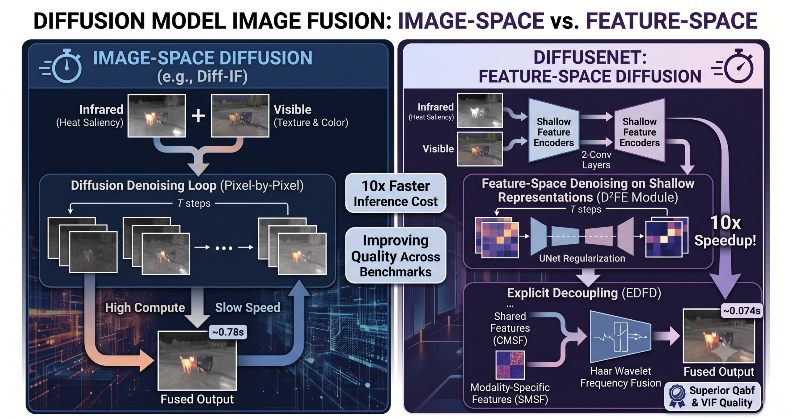
- DiffFuseNet runs diffusion denoising on shallow two layer encoded features instead of full images, cutting inference time to 0.074 seconds per pair versus 0.78 seconds for the image space diffusion baseline Diff-IF, a roughly tenfold speedup.
- The model explicitly separates shared cross modal features from modality specific features before fusion, rather than mixing everything through a single shared encoder.
- Haar wavelet decomposition combined with invertible neural networks gives lossless frequency separation, letting the network treat global structure and local texture differently.
- Across TNO, RoadScene, and M3FD benchmarks, DiffFuseNet posts the best or close to best scores on entropy, spatial frequency, and the perceptual Qabf metric.
- On downstream tasks, the fused images improve semantic segmentation mIoU to 0.7300, the best among ten compared methods, and competitive object detection recall on LLVIP.
- The model also generalizes to medical image fusion (MRI-CT, MRI-PET, MRI-SPECT) as a secondary evaluation domain, though the paper makes no clinical claims about diagnostic readiness.
The Real Problem With Fusing Infrared and Visible Images
Infrared sensors see heat. Visible sensors see texture and color under adequate light. Combine them well and you get an image where a person standing in shadow is still clearly a person, where a license plate is readable at night, where a building’s outline is visible through fog. Combine them badly and you get a muddy compromise that loses what each sensor was good at.
The paper from Wang et al., published in Pattern Recognition (2026), frames the persistent difficulty in four parts. Encoders struggle to extract clean modality specific features under low light or sensor noise. Naive combination strategies, simple addition or concatenation, let one modality dominate the other. Explicit separation of what the two modalities share versus what is unique to each is rarely done properly, which limits how adaptively a network can fuse them. And training is inherently unstable because there is no ground truth fused image to supervise against, since no camera produces a perfectly fused infrared and visible pair to learn from directly.
That last point matters more than it sounds. Most fusion networks are trained with reconstruction losses, structural similarity, and hand designed objectives because there is nothing else to anchor on. Generative adversarial approaches have tried to fill that gap but tend to suffer mode collapse, where the generator settles into producing a narrow range of outputs regardless of input variation. Spatial transformer networks assume the misalignment between modalities can be modeled with parametric warping, which breaks down when the physical discrepancy between thermal and optical imaging is not rigid (a person’s outline in infrared does not deform the same way as their outline in visible light under perspective shift).
Why Feature Space Diffusion Beats Image Space Diffusion
This is the paper’s central design decision, and it is worth understanding precisely because it explains both the quality gains and the tenfold speed advantage over the most comparable prior method.
Diffusion models work by learning to reverse a noise corruption process. You take clean data, add Gaussian noise across many steps until it becomes pure noise, then train a network to predict and remove that noise step by step. Applied directly to images, as the existing method Diff-IF does, this means iterative denoising across the full pixel grid, which is expensive. The paper reports Diff-IF at 637.65 GFLOPs and 0.78 seconds per image pair.
DiffFuseNet’s D²FE module instead applies the noise injection and denoising to features produced by a shallow shared encoder consisting of just two convolutional layers with GroupNorm and GELU activation. These are not deep semantic features. They retain substantial spatial locality and have not yet abstracted away from the pixel grid into high level concepts. Running diffusion on this representation rather than on raw pixels means the lightweight conditional UNet doing the denoising has far less to process, and you only need it to operate well enough to regularize the features toward a shared modality invariant manifold rather than to synthesize realistic image content from scratch.
Here F superscript zero is the initial shallow feature from either modality, and the noise schedule progressively corrupts it over T steps until it approaches pure Gaussian noise at the final step. A conditional UNet is trained to predict the injected noise at each timestep, conditioned on a sinusoidal positional embedding of the current step.
What Feature-Space Diffusion Actually Buys You
The paper’s authors are explicit that this design choice is not generative in the conventional diffusion sense. They describe the D²FE module as acting like a feature regularizer rather than a generative prior. The model is not trying to synthesize a plausible image from noise the way a text to image diffusion model does. It is using the noise and denoise training signal to push representations from two different sensors toward a common, robust subspace, without the adversarial instability that GANs introduce and without assuming a parametric geometric relationship between the modalities.
There is a subtlety in how the denoised features get back into the pipeline that is worth flagging because the authors address a real concern about it directly. After denoising, the enhanced feature map is fused and added back to the original image as a residual correction, not used to generate new pixel content outright.
The authors justify this by noting the shallow encoder has limited receptive fields and has not encoded highly abstract semantic concepts, so adding this feature map back functions as a learned, spatially adaptive contrast and detail enhancement, conceptually similar to ResNet’s identity mapping that lets a network refine an input incrementally rather than hallucinate new content. This is a reasonable design justification and it sidesteps a real failure mode of naive diffusion in the loop fusion, where deep abstract features get projected back into pixel space and introduce semantic artifacts that do not correspond to anything physically present in the scene.
Explicit Decoupling Tells Shared and Unique Information Apart
Once features are enhanced and aligned via diffusion, the EDFD module performs the second core operation. It explicitly splits what the two modalities have in common from what each one uniquely contributes. This sounds obvious but most prior fusion networks do not do it cleanly. A shared encoder learns a single representation and downstream fusion has to implicitly figure out which parts came from where.
The shared feature captures scene layout common to both sensors, things like where objects are positioned in the frame, the rough geometry of the scene. Modality specific features are then obtained by literally subtracting the shared component from each modality’s denoised features and refining the residual.
The visible specific feature ends up encoding textures and colors, the things a thermal camera physically cannot see. The infrared specific feature captures thermal saliency and edge information that survives in low light where the visible sensor struggles. This separation gives the network something concrete to control during fusion rather than hoping a single mixed representation sorts itself out implicitly.
Frequency Decomposition With Haar Wavelets and Invertible Networks
The third piece addresses a different axis of the problem, separating global structure from local texture, which is largely orthogonal to the shared versus modality specific split. A single level Haar wavelet decomposition losslessly splits each enhanced feature into four subbands, a low frequency component capturing global contour and energy, and three high frequency components capturing horizontal, vertical, and diagonal detail.
What makes this more than a standard wavelet fusion approach is the use of invertible neural networks to refine the subbands before fusion. The forward transformation in the invertible block splits the input into two halves and applies coupling operations.
An important detail here, and one that affects how you should think about this module’s actual cost, is that only the forward pass is used during both training and inference. The invertibility property is never exploited to run the network backward, which the authors note preserves the lossless information property of the architecture without the additional computational overhead that running the inverse transformation would require.
Bidirectional Cross-Frequency Attention
Low and high frequency information are not processed in isolation after the wavelet split. The model uses bidirectional attention so low frequency features (global structure, where the building is, where the road runs) guide high frequency enhancement via spatial attention, while high frequency features (fine edges, texture) supplement the low frequency representation via channel attention. This mutual guidance is what lets global semantics inform local detail while fine textures enrich the global structural estimate, rather than treating the two frequency bands as independent streams that get concatenated at the end without interaction.
What the Ablation Study Actually Tells You
The ablation results are the most useful part of this paper for anyone deciding whether to adapt pieces of this architecture rather than the whole thing. Six variants were tested, each removing or replacing one component while holding the rest fixed.
| Variant | EN | SF | SCD | VIF | Qabf |
|---|---|---|---|---|---|
| Without D²FE (no diffusion enhancement) | 7.14 | 13.50 | 1.65 | 0.75 | 0.52 |
| Without EDFD decoupling | 7.14 | 13.00 | 1.62 | 0.76 | 0.58 |
| Without frequency decomposition | 7.09 | 13.20 | 1.60 | 0.74 | 0.56 |
| Standard wavelet (no INN refinement) | 7.12 | 13.72 | 1.70 | 0.77 | 0.61 |
| Without bidirectional attention | 7.15 | 12.80 | 1.63 | 0.73 | 0.55 |
| One stage training (no Stage I/II split) | 7.10 | 12.90 | 1.64 | 0.72 | 0.54 |
| Full model (Ours) | 7.19 | 13.91 | 1.71 | 0.8 | 0.63 |
Two findings deserve more attention than the paper gives them in passing. First, removing bidirectional attention and replacing it with simple element wise addition creates the largest drop in spatial frequency (12.80 versus 13.91), meaning the attention mechanism is doing real work in preserving fine detail, not just marginal refinement. Second, the gap between standard wavelet and INN refined wavelet decomposition is the smallest of all six ablations on most metrics, which raises a fair question about whether the INN refinement earns its computational cost compared to the other three modules. The Qabf gap (0.61 versus 0.63) is real but modest, and a practitioner with tight compute budgets might reasonably trade that small loss for a simpler wavelet pipeline.
The diffusion module is not a generative prior here. It is a feature regularizer that pushes two sensors toward a shared modality invariant subspace without ever touching a pixel directly.
Interpretation of the D²FE design rationale in Wang et al., Pattern Recognition (2026)Benchmark Results Show Where DiffFuseNet Actually Wins
Across TNO, RoadScene, and M3FD, the pattern is consistent without being a clean sweep. The model leads or ties for the lead on entropy (EN) and spatial frequency (SF) on TNO, leads on the perceptual Qabf metric on RoadScene, and leads on both VIF and Qabf on M3FD. It does not win every metric on every dataset. CDDFuse posts a higher standard deviation on both TNO and RoadScene, and the authors address this directly rather than ignoring it.
| Method | EN | SD | SF | VIF | Qabf |
|---|---|---|---|---|---|
| Diff-IF (image-space diffusion) | 6.79 | 34.96 | 14.13 | 0.78 | 0.59 |
| CDDFuse | 6.9 | 37.2 | 14.74 | 0.79 | 0.61 |
| HaarFuse | 6.98 | 38.23 | 15.77 | 0.73 | 0.62 |
| DiffFuseNet (Ours) | 6.93 | 38.75 | 15.78 | 0.79 | 0.66 |
The explanation the authors give for the CDDFuse standard deviation gap is worth taking seriously rather than dismissing as post-hoc justification. CDDFuse tends to amplify high-frequency components aggressively to boost contrast, which inflates SD but risks halo artifacts and excess enhancement in flat regions. DiffFuseNet’s bidirectional cross frequency attention imposes a more conservative high frequency integration, prioritizing texture authenticity over raw contrast stretching. Whether you find that argument convincing depends partly on whether you trust VIF and Qabf as better proxies for perceptual quality than SD, which the broader image fusion literature generally does treat as the case, since SD measures pixel value dispersion rather than anything about structural or perceptual fidelity.
Downstream Task Performance Is Where the Argument Gets Stronger
Benchmark metrics on fusion quality are useful but somewhat self referential, since the metrics were largely designed around what fusion researchers think matters. Downstream task performance is a better test of whether the fused image is actually useful.
On the LLVIP object detection benchmark using YOLOv5, DiffFuseNet achieves 0.745 recall, second only to SwinFusion’s 0.766, with an mAP@.5 of 0.852, the second-best score behind SwinFusion’s 0.867. On semantic segmentation using SegFormer-B0, the result is more clearly favorable. DiffFuseNet achieves the highest mIoU among all ten compared methods at 0.7300, with particularly strong gains in challenging categories like bicycles, car stops, and guardrails, categories where fine edge preservation matters most for correct pixel classification.
This is a meaningful signal. A fusion method that scores well on EN and SF but does not translate to better downstream detection or segmentation would be optimizing for the wrong thing. The consistency between DiffFuseNet’s perceptual metrics and its downstream task gains suggests the architecture is preserving information that actually matters for machine vision tasks, not just information that happens to inflate one particular metric that uses no reference image.
The Computational Efficiency Story
This is arguably the paper’s strongest practical claim, and the numbers back it up clearly.
| Model | Type | FLOPs (G) | Params (MB) | Time (s) |
|---|---|---|---|---|
| ReCoNet | CNN | 0.41 | 0.007 | 0.024 |
| HaarFuse | CNN | 4.21 | 0.47 | 0.067 |
| SwinFusion | Transformer | 307.51 | 0.97 | 2.294 |
| CDDFuse | Hybrid | 22.97 | 1.79 | 1.409 |
| Diff-IF | Diffusion (image space) | 637.65 | 23.74 | 0.780 |
| DiffFuseNet | Diffusion (feature space) | 30.75 | 4.02 | 0.074 |
The FLOPs reduction from 637.65G to 30.75G against Diff-IF is roughly twenty fold, and the wall clock inference time drops from 0.78 seconds to 0.074 seconds, slightly more than tenfold. This is the practical payoff of keeping diffusion confined to shallow features rather than running it across the full image. Notably, DiffFuseNet’s inference time is also faster than CDDFuse and dramatically faster than SwinFusion, despite being a more architecturally complex pipeline than either, which speaks to how much the choice of where to apply expensive operations matters more than the raw parameter count.
It is worth being precise about what this comparison does and does not establish. DiffFuseNet is not the fastest method in the comparison set overall. ReCoNet and HaarFuse, both pure CNN approaches, are faster still. The honest framing, which the authors themselves use, is that DiffFuseNet offers a favorable position on the tradeoff between speed and quality rather than dominating on raw speed. If your deployment constraint is strictly inference latency on embedded hardware, a lightweight CNN based fusion network remains the better starting point.
This tradeoff is the same one we examined in our coverage of diffusion guided knowledge distillation, where the lesson was also that the location in the pipeline where you apply an expensive technique matters more than whether you apply it at all. Confining diffusion or attribution computation to a smaller, earlier representation rather than the full output consistently buys efficiency without giving up the benefit of the technique.
The Medical Imaging Results Deserve a Careful Read
The paper extends its evaluation to MRI-CT, MRI-PET, and MRI-SPECT fusion as a secondary domain. It is worth being precise about what this section does and does not claim. The paper reports quantitative metrics (entropy, spatial frequency, mutual information, VIF, Qabf) on public medical fusion benchmarks, and DiffFuseNet performs competitively, achieving the best EN, SF, and Qabf scores on the MRI-CT dataset and the best MI, SCD, and Qabf on MRI-PET.
What the paper does not claim, and what this article will not imply, is that these results constitute a validated clinical tool. This is architecture level benchmark evaluation using standard public datasets, not a clinical trial or a diagnostic accuracy study. The interesting technical observation here is that both diffusion based methods in the comparison, Diff-IF and DiffFuseNet, consistently rank in the top tier across the medical fusion metrics, which the authors interpret as evidence that diffusion guided feature alignment generalizes well to a different imaging domain with different noise characteristics and structural properties than the infrared and visible setting it was originally designed for. That is a reasonable architectural observation. It is not a clinical readiness claim, and any application of this or related architectures in a real diagnostic pipeline would require dedicated clinical validation well beyond what a Pattern Recognition methods paper provides.
Honest Limitations
What This Paper Does Not Fully Resolve
Alignment assumption. The authors state directly that the method assumes reasonably aligned input pairs and may degrade under severe misalignment. Real world infrared and visible camera rigs often have slight parallax or timing offsets, and how much misalignment this architecture tolerates before quality drops meaningfully is not characterized in the paper.
The INN module has a thin case for its cost versus benefit. As the ablation table shows, the gap between standard wavelet decomposition and INN refined decomposition is the smallest margin among the six tested components. The paper does not report the specific compute cost attributable to the INN refinement alone versus the rest of the EDFD module, making it hard to judge whether this component is worth its complexity in a deployment with limited resources.
Extreme weather untested. The authors explicitly flag that robustness under extreme weather conditions, heavy rain, dense fog at long range, or sensor degradation beyond what TNO, RoadScene, and M3FD capture, requires further validation. This matters directly for the surveillance and autonomous driving use cases the introduction cites.
No unpaired or video extension yet. The current method operates on paired, static infrared and visible frames. Extending to unaligned pairs or temporally consistent video fusion is listed as future work, not something the current architecture handles.
Hyperparameter sensitivity testing used a reduced training budget. The sensitivity analysis on loss weights was run for only 20 epochs (versus 120 for the main results) due to computational constraints. The conclusion that the model is robust to hyperparameter perturbation is reasonable given the small observed variance, but it rests on a shorter training regime than the full reported results, which is a meaningful caveat for anyone trying to reproduce the paper’s headline numbers exactly.
A Reproducible PyTorch Sketch of the D²FE Module
Below is a focused implementation of the feature space diffusion module, the architectural piece most likely to be useful in isolation for other fusion or cross modal alignment work. It includes the shallow encoder, the forward noise process, the conditional UNet denoiser, the fusion network, and a smoke test on dummy paired images.
Where This Fits in the Broader Landscape of Diffusion for Vision
The paper situates itself against two categories of prior diffusion work, feature caching acceleration methods like TaylorSeer and Spectrum, and unified multimodal generative frameworks like Transfusion and Show-o. Both categories are doing something fundamentally different from what DiffFuseNet does. Feature caching methods speed up single modal generation by reusing computation across denoising steps, but they were not designed to align two different sensor modalities at all. Unified multimodal frameworks generate fused content through iterative denoising in image space, applying the same diffusion process to both modalities homogeneously, which the authors argue fails to model the feature level discrepancies that actually distinguish infrared from visible imaging.
DiffFuseNet’s contribution sits in a narrower, more specific niche than either of those directions. It does not try to be a general purpose multimodal generator. It uses diffusion as a targeted regularization tool for a specific two modality alignment problem, and that narrower scope is exactly what allows the architecture to be lightweight enough to run at 0.074 seconds per pair. If you are exploring where diffusion models add genuine value versus where they are an expensive default, our analysis of sample level adaptive distillation for video models makes a related point from a different angle. Matching the cost of an expensive technique to the part of the problem that actually needs it, rather than applying it uniformly, is consistently where the practical gains show up.
Frequently Asked Questions
Read the full paper and access the published version through Pattern Recognition.
Read via DOI View on ScienceDirectClosing Thoughts
DiffFuseNet is a well built answer to a specific, well posed question. Can diffusion models contribute to image fusion without the computational cost that has limited their practical deployment in this domain. The answer the paper gives is yes, provided you are willing to confine the diffusion process to a narrow, well defined regularization role rather than asking it to do generative heavy lifting.
The architecture combines that insight with two other solid ideas, explicit decoupling of shared and modality specific information, and frequency aware fusion via wavelets and invertible networks, both of which the ablation study supports as meaningful contributors rather than decorative additions. The bidirectional cross frequency attention component in particular earns its place in the architecture based on the ablation evidence.
Where the paper is appropriately cautious is in acknowledging what remains unresolved. The alignment assumption, the untested extreme weather robustness, and the relatively thin case for the INN cost versus benefit tradeoff are all real gaps the authors name rather than gloss over. That honesty is worth noting, particularly in a subfield where overclaiming about diffusion model benefits has become common.
The most transferable lesson here extends beyond infrared and visible fusion specifically. When considering whether to add diffusion based regularization to any cross modal alignment problem, the relevant design question is not whether diffusion helps, since in some form it usually does, but where in the pipeline you can apply it cheaply enough that the benefit outweighs the cost. DiffFuseNet’s answer, push it as early and as shallow as the architecture will tolerate, is a template worth testing in other multimodal settings beyond image fusion.
Related Articles
This analysis is based on the published paper and an independent evaluation of its claims. This article makes no clinical or diagnostic claims regarding the medical imaging benchmarks discussed.