Key points
- Vision RWKV offers the linear complexity that transformers cannot match at high resolution, but its recurrent horizontal and vertical scanning introduces a directional bias the authors trace to a Bayesian argument.
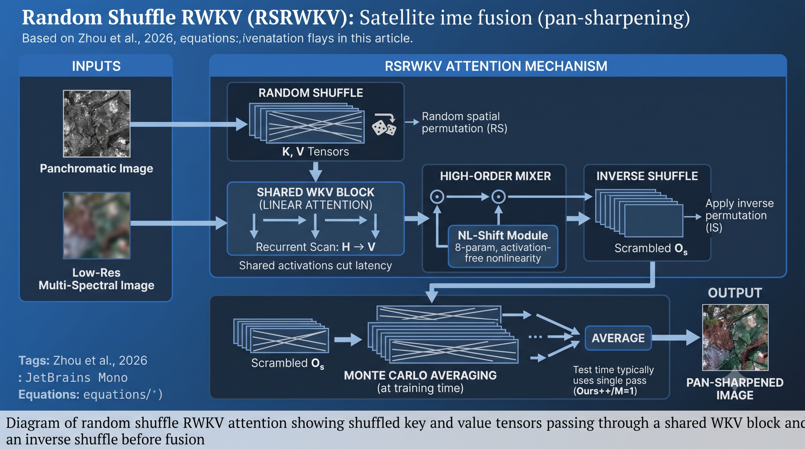
- Random Shuffle RWKV, shortened to RSRWKV, scrambles the scan order before attention and reverses it afterward, then averages several shuffled passes at test time the way Monte Carlo dropout does.
- A WKV sharing mechanism reuses attention activations across layers to cut latency, while a redesigned channel mixer pushes the model from first order to higher order feature interaction.
- A max pooling step reinjects high frequency detail that linear attention naturally smooths away, and a lightweight NL-Shift module adds nonlinearity with only eight extra parameters.
- A new manifold loss built on Taylor expansion with randomly reinitialized weights replaces fixed wavelet or Fourier losses, and the full system beats fifteen published baselines on three satellite datasets.
Why fusing a sharp photo with a blurry one is harder than it sounds
Pan sharpening takes two pictures of the same ground scene captured by the same satellite. One is panchromatic, a single grayscale channel with fine spatial detail, sharp edges, and true resolution. The other is multi spectral, several color channels that carry the actual spectral information a scientist cares about, but captured at a much coarser resolution because more channels means less light per pixel. The goal is to merge them into one image that has the spatial sharpness of the panchromatic shot and the spectral fidelity of the multi spectral one, without inventing detail that was not really there or smearing colors that should stay distinct.
For years this was solved with classical signal processing, methods like intensity hue saturation fusion, principal component analysis, and the Brovey transform, which the paper groups under component substitution. A second family called multi resolution analysis attacks the problem in frequency space, and a third called variational optimization writes the whole thing as an energy minimization problem with hand tuned constraints. All three approaches work reasonably well and none of them require training data, which is a real advantage, but they tend to introduce artifacts, spectral distortion, or both, especially on scenes with fine texture.
Convolutional networks changed that starting with Masi and colleagues applying a plain CNN to the problem, and a long line of work since then has added residual blocks, multi scale inputs, and physics informed priors borrowed from the variational literature. More recently, transformer based fusion networks like SwinFusion pushed performance further by modeling long range spatial relationships, the kind of relationship a small convolution kernel simply cannot see. The catch is well known to anyone who has tried to run a vision transformer on a full resolution satellite tile. Attention costs grow with the square of the number of pixels, and a modern multi spectral scene can easily have enough pixels to blow past the memory of a single GPU before training even gets underway.
RWKV as a way around the memory wall
RWKV began as a language model architecture built to match transformer quality with the training efficiency of a recurrent network, and it has since been adapted for vision tasks under names like vision RWKV. The trick is a component called WKV, short for a weighted key value computation, which behaves like linear attention. Instead of computing a full pairwise similarity between every pixel and every other pixel, which is what standard softmax attention does and why its cost scales quadratically, WKV accumulates information through a recurrent scan across the sequence, which scales linearly with the number of pixels. Figure 1 of the paper shows this difference in stark terms. Past a modest resolution the transformer baseline runs out of memory entirely, while the RWKV based approach keeps running with modest and gradually increasing cost.
Linear complexity is not free, though. To model two dimensional spatial relationships with a mechanism built for one dimensional sequences, vision RWKV has to unroll the image into a sequence, typically scanning horizontally then vertically, and it does this recurrently across several iterations to approximate full two dimensional coverage. That scanning order is fixed by construction. Every image gets read in the same direction every time, which is exactly the kind of arbitrary, unjustified choice that tends to leak into what a model learns.
The Bayesian argument for why fixed scanning is biased
The authors frame the scan order as a latent variable rather than an architectural detail. In their words, treat the specific scanning sequence as a random variable and ask what the true output should be if you marginalized over every possible scanning order, weighted by how plausible each order is. A model that always uses the same one fixed order is implicitly assuming that order deserves all of the probability mass and every other order deserves none, which is an arbitrary prior with no justification in the actual geometry of an image. Two dimensional spatial dependencies have no privileged direction. A pixel’s relationship to its neighbor above should not be modeled any differently than its relationship to its neighbor to the left, yet a fixed sequential scan effectively treats them differently by construction.
Random shuffle, the fix that borrows from Dropout
The proposed remedy is almost disarmingly simple to state even though the justification behind it runs deep. Before feeding the key and value tensors into the WKV computation, randomly permute their spatial order using a random index generator. Run the attention computation on the shuffled sequence. Then apply the inverse of that same permutation to put every feature back exactly where it started, a step the authors call inverse shuffle. Because the shuffle and its inverse are exact opposites of each other, the operation preserves what the paper calls information coordination invariance, meaning nothing about the content changes, only the order in which the recurrent scan encounters it.
Here RS is the random shuffle function and IS is the corresponding inverse shuffle. Because a single random draw only samples one of an enormous number of possible orderings, the authors reach for the same logic behind Dropout at test time. Rather than trust any one shuffled pass, they treat the true output as the expected value over the full distribution of shuffling permutations and approximate that expectation with Monte Carlo averaging, running the same input through several independently shuffled forward passes and averaging the results.
A natural worry here is that averaging several forward passes multiplies inference time by that same factor. The paper addresses this directly and rather elegantly. Since each shuffled pass is independent, the multiple runs can be packed into a single mini batch of repeated copies of the same input and processed simultaneously on modern accelerators, so the wall clock cost barely moves even though the arithmetic cost technically increases. An ablation in Figure 14 goes further and shows the practical punch line. PSNR stays essentially flat whether the model averages one sample or thirty two, hovering around 42.0944 to 42.0950 dB across the whole range they tested, so the authors settle on using a single sample at test time, which means the debiasing benefit of random shuffle comes essentially for free at inference once the model has been trained with the strategy.
Sharing attention instead of recomputing it, and going beyond first order
A second structural contribution addresses a completely different inefficiency. Standard RWKV blocks recompute their key value attention scores fresh at every layer, which the authors argue is wasteful once you look at what those activations actually represent. The paper introduces WKV sharing, where the attention output computed at one layer is directly reused at the next rather than recalculated from scratch, cutting the redundant computation and, according to the ablation in Figure 16, meaningfully reducing latency and improving how easily the network trains.
The more conceptually interesting move is what the paper calls high order modeling. It starts from an observation about what attention actually is mathematically. The sigmoid gated combination used in RWKV’s spatial mixer, written as the elementwise product of a sigmoid gate and the WKV output, satisfies the two defining properties of a probability distribution, values bounded between zero and one that sum to one across the relevant dimension. That means the whole attention operation is mathematically equivalent to computing a first order statistical expectation over the value tensor. Once you see attention as an expectation calculation rather than a bespoke architectural trick, a natural question follows. Most existing methods that try to capture richer, higher order interactions do it by cascading several of these first order operations one after another, which the paper shows is really only capturing repeated second order effects stacked in sequence, an approach that is both computationally expensive and structurally limited.
Instead of stacking, the paper proposes sharing the gating mechanism itself across layers in the channel mixer, which lets the network build genuinely higher order interactions without paying for a deeper cascade. The channel mixer’s original design used a sigmoid gate to scale value features. Combined with the activation free philosophy discussed next, the authors strip that gate out entirely, arguing the sigmoid nonlinearity was constraining information flow more than it was helping, and replace it with a simpler and more expressive elementwise product.
Removing activation functions on purpose
The paper leans into a design philosophy the authors call activation free, extended here from prior work on simple image restoration baselines. The general move is to take an operation of the form one function times an activation applied to a second function, and simplify it to just the two functions multiplied together, dropping the nonlinearity in between. Applied to the channel mixer, this removes the sigmoid gate. Applied to a component called Q-shift, a small depth wise three by three convolution kernel that mixes information from neighboring pixels along the channel dimension, activation free thinking runs into a genuine tension. Simply enlarging the kernel to capture more context, the approach earlier papers tried, brings back exactly the parameter growth the activation free philosophy was trying to avoid.
The paper’s answer is a new module called NL-Shift, which restores meaningful nonlinear representation capacity while adding only eight parameters total, one learnable weight and one bias per channel group across four channel split groups. Structurally it applies layer normalization, then the shift operation, then multiplies that shifted and normalized result back against another normalized copy of the input, an elementwise trick that introduces genuine nonlinearity without introducing an activation function or meaningfully increasing the parameter count.
Fighting the low pass tendency of linear attention
Linear attention mechanisms including WKV have a known mathematical tendency to behave like a low pass filter, smoothing away exactly the high frequency detail that pan sharpening depends on for spatial sharpness. The paper cites prior Fourier domain analysis establishing this property formally and responds with a genuinely simple fix, a max pooling layer inserted to actively extract and reinject high frequency components that would otherwise get smoothed away.
The ablation results back this up concretely. Removing the anti low pass mechanism from the full model costs measurable PSNR across all three test datasets, and a Fourier amplitude visualization in Figure 19 shows the reinjected features carry visibly more high frequency energy than the version without the max pooling step.
A loss function built from an infinite family of constraints
Pan sharpening papers have historically supervised their networks with fixed frequency domain losses, penalizing the difference between predicted and ground truth images after a discrete wavelet transform or a discrete Fourier transform. Both of those transforms use a single fixed orthogonal basis, which the authors argue introduces its own bias, since a fixed basis cannot capture the full complexity of how prediction errors are actually distributed relative to the ground truth.
Their alternative draws on a different piece of theory entirely, Taylor’s unfolding manifold, previously used in a deep Taylor approximation framework where one network branch learns the main, low frequency energy of an image and a second branch built from shared derivative function weights progressively recovers finer, higher order detail. The new twist here is randomization. Rather than using one fixed set of weights for that Taylor expansion, the weights are reinitialized randomly at the start of every training epoch, drawn from standard schemes like Xavier initialization, Kaiming initialization, or a plain Gaussian distribution.
Conceptually, the paper describes the traditional fixed basis approach as a single point constraint, one specific way of decomposing the image that the loss enforces every single time. Randomizing the weights of the Taylor manifold on every epoch means each training step effectively samples a different, but related, decomposition of the same underlying reconstruction problem, which the authors argue amounts to an infinite family of point constraints rather than just one, tightening the effective solution space the network is allowed to settle into over the course of training without ever committing to any single fixed transform.
Why this framing matters beyond pan sharpening
The general pattern, replacing one fixed transform based loss with an ensemble of randomly reinitialized functional constraints applied over training, is not tied to satellite images specifically. Anywhere a fixed wavelet or Fourier penalty is used to encourage sharper reconstructions, whether in super resolution, denoising, or general image restoration, this same randomization idea could plausibly transfer, though the paper only tests it here.
How it actually performs against the field
The team benchmarked against five classical methods, SFIM, Brovey, GS, IHS, and GFPCA, and fifteen deep learning baselines including PNN, PanNet, MSDCNN, SRPPNN, GPPNN, MutNet, SFINet, SHIP, PanFlowNet, ADWM, TMDiff, DISPNet, BUGPan, WaveLetNet, and CFHIPS, across three satellite platforms, WorldView-II, GaoFen2, and WorldView-III.
Reduced resolution results, where ground truth is simulated
| Dataset | Method | PSNR up | SSIM up | SAM down | ERGAS down |
|---|---|---|---|---|---|
| WorldView-II | Best baseline, SHIP | 42.1357 | 0.9726 | 0.0212 | 0.9047 |
| Ours | 42.0945 | 0.9721 | 0.0214 | 0.9081 | |
| Ours++ | 42.3479 | 0.9736 | 0.0209 | 0.8834 | |
| WorldView-III | Best baseline, WaveLetNet | 30.9139 | 0.9279 | 0.0710 | 2.9770 |
| Ours | 30.9665 | 0.9266 | 0.0726 | 2.9247 | |
| Ours++ | 31.1342 | 0.9277 | 0.0716 | 2.9221 | |
| GaoFen2 | Best baseline, SHIP | 47.6369 | 0.9897 | 0.0099 | 0.5272 |
| Ours | 47.7144 | 0.9896 | 0.0098 | 0.5229 | |
| Ours++ | 47.8379 | 0.9899 | 0.0096 | 0.5175 |
GaoFen2 is the cleanest sweep, with the enhanced Ours++ model beating every baseline on every one of the four reported metrics, PSNR, SSIM, spectral angle mapper, and relative dimensionless global error. WorldView-II is nearly as clean. WorldView-III is the one place where the numbers are genuinely mixed rather than a clean sweep. WaveLetNet actually posts a slightly better structural similarity score, 0.9279 against 0.9277, and a slightly better spectral angle, 0.0710 against 0.0716, even though Ours++ wins convincingly on the headline PSNR and ERGAS metrics. That is worth noting rather than glossing over, since a genuinely honest read of the table shows this is not a total sweep on every dataset, even if the overall picture clearly favors the proposed method.
Full resolution, real sensor conditions with no simulated ground truth
Reduced resolution testing relies on the Wald protocol, which manufactures a pseudo ground truth by degrading a real high resolution image, a necessary compromise since no one has a genuinely higher resolution reference to compare against. Full resolution testing skips that simulation and evaluates directly on the original sensor data, scored with no reference metrics since there is no ground truth to compare against at all, specifically QNR, a composite quality index, alongside its two distortion components.
| Dataset | Best baseline | Baseline QNR | Ours QNR | Baseline spectral distortion | Ours spectral distortion |
|---|---|---|---|---|---|
| WorldView-II | ADWM | 0.7921 | 0.7958 | 0.0955 | 0.0934 |
| GaoFen2 | ADWM | 0.8307 | 0.8345 | 0.0682 | 0.0650 |
Here the proposed model comes out ahead of every listed baseline, including transformer based INNformer and flow based Panflow, on the composite QNR score for both datasets, which is a meaningful result since full resolution behavior is arguably closer to how the model would actually perform once deployed against a real satellite feed rather than a laboratory simulation of one.
What happens as the network gets deeper
| Configuration | Layers L | PSNR | SSIM | SAM | ERGAS |
|---|---|---|---|---|---|
| Tiny | 3 | 41.9596 | 0.9715 | 0.0220 | 0.9133 |
| Small | 7 | 41.9972 | 0.9716 | 0.0218 | 0.9184 |
| Regular | 9 | 42.0945 | 0.9721 | 0.0214 | 0.9081 |
| Large | 11 | 42.0976 | 0.9722 | 0.0213 | 0.9076 |
Going from three layers to nine buys a real, if modest, improvement, but pushing further to eleven layers barely moves any metric. The team settled on nine layers as their default, a sensible tradeoff between the diminishing accuracy returns and the added compute of a deeper stack.
What each new component actually buys you
Section 4.6 of the paper runs a genuinely useful set of ablations that isolate each of the three components added beyond the earlier conference version of this work, which the authors call Ours in these tables, with the fully assembled model called Ours++.
| Configuration removed | WorldView-II PSNR | WorldView-III PSNR | GaoFen2 PSNR |
|---|---|---|---|
| Baseline, Ours | 42.0945 | 30.9665 | 47.7144 |
| Without anti low pass | 42.2468 | 31.0157 | 47.7614 |
| Without activation free channel mixer | 42.1816 | 30.8895 | 47.6623 |
| Without NL-Shift | 41.9903 | 30.7431 | 47.5216 |
| Full model, Ours++ | 42.3479 | 31.1342 | 47.8379 |
Removing NL-Shift is the one that hurts the most, dropping WorldView-II performance below even the earlier baseline model, which tracks with the paper’s own description of it causing the most noticeable decline and visibly blurred texture boundaries in the accompanying figures. Removing the activation free channel mixer causes a smaller but consistent drop paired with slight color distortion in the visual comparisons. Removing anti low pass causes the smallest individual drop of the three, which makes sense given it addresses a comparatively narrower problem, the tendency of linear attention specifically to blur fine texture, though the ablation in Figure 16 covering the earlier core designs, WKV sharing, the channel mixer cache, random shuffle itself, and the manifold loss, found every one of those four components was necessary too, with removing random shuffle in particular reintroducing the fixed sequence bias the whole paper set out to solve in the first place.
Reading the receptive field visualizations honestly
Figure 11 in the paper compares effective receptive field visualizations across convolution, self attention, transposed attention, window attention, and the proposed random shuffle RWKV, with the described intent that a wider spread of intense color represents a larger and more globally aware receptive field. RSRWKV is described as covering the widest area of any method compared, consistent with the paper’s central claim that linear complexity attention can still capture genuinely global context rather than trading receptive field size for computational savings.
Honest limitations
A few things are worth naming plainly rather than leaving implicit. This is a fairly fresh publication, appearing online in June 2026, and it substantially extends an earlier NeurIPS 2025 conference paper by the same core authors, so some of the foundational random shuffle and WKV sharing ideas have had at least one round of prior peer review, while the newer NL-Shift, activation free channel mixer, and full ablation results in this journal version are more recent. The WorldView-III comparison shows the method does not universally dominate every single metric against every single baseline, WaveLetNet edges it out narrowly on structural similarity and spectral angle there, a detail easy to miss if you only read the abstract’s framing of consistent state of the art results. The evaluation is also confined to three specific commercial satellite platforms and their particular sensor characteristics, and all training relies on the Wald protocol for reduced resolution ground truth, a widely accepted but still simulated proxy rather than genuinely higher resolution imagery. Finally, the Monte Carlo random shuffle strategy at training time adds computational overhead beyond a single fixed scan, and while the authors show inference cost stays low by batching shuffled copies together, training cost was not broken out separately from the baseline vision RWKV architecture in the reported numbers.
Takeaway for practitioners
If you already have a vision RWKV pipeline running into directional bias or blurred high frequency detail, the random shuffle and inverse shuffle pairing is a genuinely lightweight change to try first, since it needs no additional parameters, only a random permutation and its inverse applied around the existing WKV block.
Takeaway on the theory
The framing of attention as a first order statistical expectation, and higher order interaction as sharing that expectation’s gating mechanism across layers rather than cascading more of it, is a genuinely useful lens that could inform other linear attention designs well beyond pan sharpening specifically.
Where this could go next
The specific achievement here is narrow, a better way to fuse a panchromatic and a multi spectral satellite image. The idea underneath it is not narrow at all. Treating a fixed scanning order inside a sequential attention mechanism as an unjustified prior, and correcting for that prior with a randomization and inverse randomization pair borrowed from Bayesian reasoning, is a technique that could plausibly transfer to any vision task built on a recurrent or state space style attention mechanism, not just RWKV and not just satellite imagery. Medical image segmentation, video understanding, and general purpose image restoration all use architectures that impose some kind of fixed traversal order on two dimensional data, and all of them could in principle carry the same hidden directional bias this paper identifies.
The manifold loss idea is similarly portable. Any restoration task currently relying on a fixed wavelet or Fourier penalty to encourage sharper output could in principle swap in a randomly reinitialized functional constraint instead, though whether the gains generalize outside pan sharpening remains untested here. The authors themselves frame extending the framework to other image processing tasks and further probing its theoretical properties as future work rather than a settled question.
What is already settled, at least within the scope of these three datasets, is that treating scan order as a statistical nuisance parameter to be marginalized away, rather than an architectural given to be accepted, produces a measurable and mostly consistent improvement over a strong and recent set of published baselines, while keeping the linear complexity that made RWKV attractive in the first place.
Read the full paper for the complete derivation of the manifold loss, all five ablation figures, and the visual comparisons across every dataset.
A minimal PyTorch implementation
Below is a compact, runnable sketch of the core ideas, a random shuffle and inverse shuffle pair around a simplified WKV block, WKV sharing across two layers, an NL-Shift module, and a manifold style loss with randomly reinitialized weights. It favors clarity over matching the paper’s exact backbone, and it includes a smoke test on random dummy data.
Conclusion
The core achievement of this paper is a fix for a bias that had been sitting quietly inside vision RWKV attention the whole time, hidden in the assumption that any single scanning direction was a neutral, harmless implementation detail rather than an implicit and unjustified statistical prior. Reframing scan order as a latent variable to be marginalized over, rather than a fixed architectural choice, gives the authors a principled reason to shuffle and unshuffle the sequence around the attention computation, and the Monte Carlo framing at test time means that debiasing step costs almost nothing once inference is batched sensibly.
The conceptual shift worth carrying forward is broader than pan sharpening. Any architecture that imposes a fixed traversal order on inherently unordered or multi directional data, whether that is an image, a point cloud, or some other spatial structure, is making the same kind of implicit assumption this paper identifies and corrects. The idea of treating that assumption as a random variable to marginalize away, rather than a hyperparameter to tune, is a genuinely transferable piece of thinking, independent of whether the underlying attention mechanism happens to be RWKV specifically.
The manifold loss contributes a second, related idea in the same spirit, that a fixed transform based loss function is itself a kind of hidden bias, and that randomizing the transform across training steps can regularize the solution space more thoroughly than committing to any single fixed basis ever could. Both ideas share a common thread, replacing a single fixed choice with a randomized ensemble of equally valid choices, evaluated in expectation rather than committed to individually.
Set against those conceptual contributions, the concrete limitations are manageable rather than disqualifying. The WorldView-III results are not a clean sweep, the evaluation covers three specific commercial satellite platforms rather than a broader remote sensing benchmark, and the added computational cost of shuffling and unshuffling, while shown to be manageable through batching, is real. None of that undercuts the central result, that a linear complexity attention mechanism can be debiased against directional preference without sacrificing the speed advantage that made it attractive in the first place, while simultaneously outperforming both the quadratic transformer baselines it was built to replace and a wide field of purpose built pan sharpening networks.
Whether this becomes a standard technique across other RWKV based vision applications or stays a pan sharpening specific contribution will depend on whether follow up work tests the random shuffle idea on the broader set of tasks the authors themselves flag as future work. The theoretical argument behind it, grounded in a fairly basic Bayesian marginalization idea, applies well beyond satellite image fusion, which is reason enough to expect this specific paper will not be the last place the idea shows up.
Frequently asked questions
What is pan sharpening in remote sensing
It is the process of combining a high resolution grayscale panchromatic satellite image with a lower resolution multi spectral image of the same scene to produce a single output that has both the spatial sharpness of the panchromatic image and the color and spectral detail of the multi spectral image.
What is the directional bias problem in vision RWKV
Vision RWKV scans an image in a fixed sequence, typically horizontally then vertically, to approximate two dimensional attention using a mechanism built for one dimensional sequences. The paper argues this fixed scanning order acts as an unjustified statistical prior, since two dimensional spatial relationships in an image have no inherently privileged direction.
How does random shuffle RWKV fix that bias
It randomly permutes the spatial order of the key and value tensors before the WKV attention computation, runs the attention on that shuffled sequence, then applies the exact inverse permutation afterward to restore the original spatial order. At test time it can average several independently shuffled passes, similar in spirit to Monte Carlo dropout, though the paper finds a single pass is usually sufficient in practice.
Does averaging multiple shuffled passes slow down inference
The paper shows the multiple passes can be batched together and run concurrently on modern accelerators, so the wall clock cost stays low. Their own ablation also found that performance is stable whether one sample or thirty two samples are averaged, so they use a single sample by default at test time.
What is NL-Shift and why does it matter
NL-Shift is a redesigned version of a component called Q-shift that adds meaningful nonlinear representation capacity using only eight additional parameters, one learnable scale and one bias per channel group across four groups. The ablation study found removing it caused the largest single performance drop of any tested component.
Does this method beat every baseline on every dataset
Mostly, but not universally. On GaoFen2 and WorldView-II the proposed model beats every listed baseline across all four reported metrics. On WorldView-III, a competing method called WaveLetNet posts a marginally better structural similarity score and spectral angle mapper score, even though the proposed model still wins on the headline PSNR and ERGAS metrics there.
Zhou, M., Li, X., He, X., Zhao, M., Qi, Y., Hong, D., and Huang, B. Random shuffle high order RWKV for pan sharpening. Information Fusion, volume 136, 2026, article 104545, DOI 10.1016/j.inffus.2026.104545. This analysis is based on the published paper and an independent evaluation of its claims.