
Key points
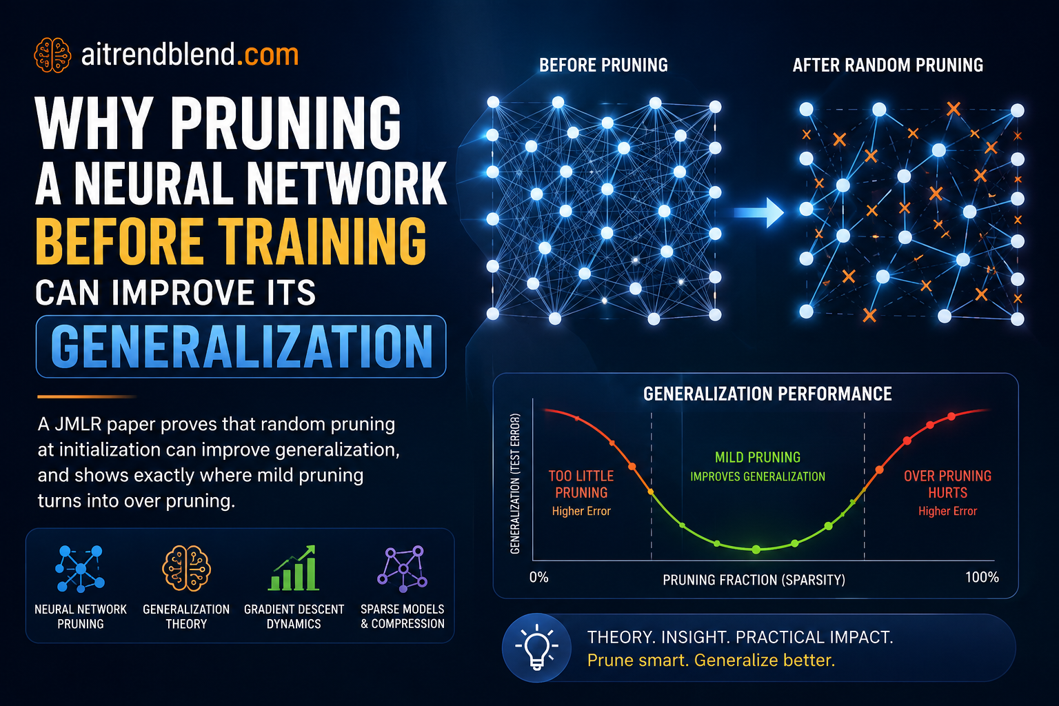
- Researchers from the University of Texas at Austin, Ohio State University, and IBM proved the first theoretical result explaining why random pruning at initialization sometimes beats the full dense network on test accuracy.
- The paper identifies two regimes. Mild pruning preserves the signal a network needs to learn while cutting noise, which improves the generalization bound as the pruning fraction grows within that range.
- Push the pruning fraction past a second threshold and the story flips. The network still drives its training loss to zero, yet its test performance collapses to roughly the level of random guessing.
- The analysis works in the feature learning regime rather than the neural tangent kernel regime, meaning the network weights are allowed to travel far from where they started, which is closer to how real networks train.
- Experiments on MNIST, CIFAR-10 with VGG-16, and ResNet architectures back up the theory qualitatively, even though the formal setup is a simplified signal and noise classification task.
A question that empirical results kept raising but nobody had answered
Anyone who has spent time pruning networks has probably run into this pattern. You strip away a chunk of weights before training even starts, retrain the smaller network, and the test accuracy comes back close to the original, sometimes a hair better. Frankle and Carbin’s lottery ticket hypothesis from 2018 gave this phenomenon a name and sparked an entire subfield chasing the sparse subnetworks hiding inside dense ones at initialization. What followed was a wave of increasingly clever ways to find those subnetworks, using loss gradients, connection sensitivity scores, or synaptic flow.
Then a strange thing happened. Researchers kept discovering that random pruning, no clever selection criterion at all, could match or even beat the fancier methods in a surprising number of cases. That is unsettling if your mental model says pruning works because you found the “right” weights to keep. If a coin flip for each weight does nearly as well, the explanation for why pruning helps generalization at all probably has nothing to do with picking winners and everything to do with how training itself changes once part of the network is missing.
That is the gap this paper by Hongru Yang, Yingbin Liang, Xiaojie Guo, Lingfei Wu, and Zhangyang Wang steps into. Their framing is refreshingly narrow and useful because of it. Rather than trying to explain every empirical pruning result at once, they ask one focused question. How does the fraction of weights you prune change the trajectory of gradient descent, and what does that trajectory imply for how the trained network will perform on new data.
Why the neural tangent kernel view could not answer this
Most of the theoretical machinery available for analyzing over parameterized networks comes from the neural tangent kernel line of work, where a sufficiently wide network behaves almost like its own linear approximation around initialization. That is a powerful simplification, and it is also exactly why it cannot explain this phenomenon. In the kernel regime the weights barely move from where they started, so a naive argument about pruning at initialization would say pruning simply throws away a random slice of both the useful signal correlation and the noise correlation in roughly equal proportion. Averaged over all the neurons, that argument concludes pruning can only hurt, never help.
The paper walks through exactly that misleading argument in detail before dismantling it. At initialization, summing the signal correlation across every neuron shows pruning shrinks the total signal strength by a factor tied to the pruning probability itself, while the noise strength shrinks by a smaller factor tied to its square root. On paper that says pruning should always hurt the signal more than the noise. If you stopped the analysis there, you would conclude pruning can never be a good idea, which flatly contradicts what practitioners keep observing.
The minimal setting the authors built to make the question tractable
Data made of a sparse signal buried in noise
To get a clean answer, the authors do not try to model images or language. They build the simplest data distribution that still captures the essential tension a real classifier faces, separating a true signal from irrelevant noise. Each class gets its own signal vector. A training example is built from two halves. One half carries the class signal, the other half carries pure Gaussian noise, and which half gets which is randomized per example. This mirrors an observation from real networks, where activations after a ReLU layer tend to be sparse, so only a subset of neurons fire for any given input, and different classes tend to activate different neurons.
They also point out why the sparsity assumption on the signal matters and is not just a convenience. If the signal were spread evenly across every coordinate instead of concentrated, pruning would shrink the signal and the noise by the same factor, and the entire mild pruning effect the paper is built around would disappear. The concentrated, sparse structure of the signal is precisely what lets pruning hit the noise harder than the signal.
A small convolutional network, pruned exactly once
The network itself is a two layer convolutional model using a polynomial ReLU activation, cubing the usual rectified output rather than leaving it linear. That choice is a deliberate analytical convenience borrowed from prior feature learning papers. A cubic nonlinearity separates neurons that are correlated with signal from neurons that are only picking up noise far more sharply than a plain ReLU would, which makes the proof tractable while the authors argue the qualitative story carries over to ordinary ReLU networks.
A binary mask is drawn once, with every entry an independent coin flip that keeps a weight with probability p, and that mask never changes again during training. This is the random pruning setup, not iterative magnitude pruning, and not a learned mask. Every neuron that fails to receive any connection to its class signal after pruning falls into what the paper calls the noise set, meaning it can only ever learn from noise no matter how long training runs. As pruning gets more aggressive, more neurons fall into that noise set, which is the seed of the over pruning failure mode described later.
How mild pruning provably helps, in three stages
The proof tracks gradient descent through three phases, and each phase tells part of the story.
Stage one, initialization
Before any training happens, the paper proves a precise bound. With mild pruning, the strongest signal correlated neuron in each class still has a correlation with its class signal that is barely reduced from the unpruned case. Meanwhile the strongest noise correlated neuron has its correlation with any particular noise vector reduced by a factor tied to the square root of the pruning rate. In plain terms, pruning knocks the noise down harder than it knocks the signal down, as long as there are enough neurons per class for at least one of them to still get lucky and land near the signal.
Stage two, the feature growing phase
Once training starts, gradient descent does not treat every neuron equally. The cubic nonlinearity means neurons that start out with even a small edge in signal correlation get a disproportionately large gradient push, so that edge compounds quickly. The paper proves that within a bounded number of steps, at least one neuron per class reaches a strong correlation with its class signal, on the order of the inverse of the network width raised to a small power, while the correlation with noise and with other classes stays provably small throughout this phase. This is the feature learning regime the authors keep contrasting with the neural tangent kernel picture. Weights are moving far from initialization on purpose, and pruning is shaping which direction they move in.
Stage three, the converging phase
The final phase drives the training loss down to whatever target threshold you set, while the signal correlation gained in stage two survives largely intact and the noise correlation stays bounded by that same square root of p factor from initialization. Proving this required the authors to build a new gradient bound for cross entropy loss across many classes rather than only two, since most of the earlier feature learning literature only handled binary classification. Getting that bound tight enough to avoid picking up an extra cubic factor in the number of classes turned into one of the more technical contributions of the paper, using the fact that the gradient contributions across the wrong classes have to sum to the same magnitude as the gradient on the correct class.
What happens when pruning goes too far
The paper’s second main theorem is the sobering half of the story. Push p small enough and the picture inverts almost completely. At that pruning fraction, the probability that a given class receives no signal at all in any of its neurons becomes overwhelming. With no way to learn the actual signal, gradient descent does something a classifier can still technically do, which is memorize the specific noise vectors in the training set well enough to drive the training loss to zero anyway. High dimensional Gaussian noise vectors are nearly orthogonal to each other, so a network with enough neurons can carve out a separate response for each training example’s noise pattern without ever learning anything that would transfer to a new, unseen example.
The generalization loss the paper proves for this regime lands at roughly the loss you would get from guessing among the classes uniformly at random. Training accuracy near perfect, test performance no better than a coin flip scaled by the number of classes. That is a much more dramatic failure than simply saying pruning hurts a little. It is a demonstration that the usual explanation for pruning failures, that the network becomes too small to represent the function it needs, is not the whole story here. The network in this regime is perfectly capable of hitting zero training loss. What breaks is the direction gradient descent travels once the signal path is cut off.
| Regime | Pruning fraction (keeping probability p) | Training loss | Generalization behavior |
|---|---|---|---|
| Full dense network | p equals 1, nothing pruned | Driven to near zero | Baseline generalization set by the noise level in the data |
| Mild pruning | Above a threshold on the order of log d divided by the network width | Driven to near zero | Generalization bound improves as p decreases within this range, meaning modest additional pruning helps |
| Over pruning | On the order of one divided by the number of classes, the width, and log d | Still driven to near zero | Generalization loss approaches the level of random guessing across the classes |
Checking the theory against MNIST, CIFAR-10, and real architectures
A theory built on a stylized signal and noise distribution earns extra scrutiny when it claims relevance to practice, and the authors clearly know that. Their simulations start close to the theoretical setting, with a binary classification task built from a signal vector plus Gaussian noise, and they show the pattern predicted by the theory. At a moderate noise level, testing error stays flat or improves as the pruning rate grows up to around half the weights, then rises sharply once pruning passes that point, all while training accuracy stays essentially perfect the entire time.
They then move to architectures people actually use. On a two layer MLP with 1024 units per layer trained on MNIST, test accuracy tracks the dense network closely up to roughly 79 percent sparsity before falling off. On VGG-16 trained on CIFAR-10, that comfortable range is noticeably narrower, holding up to about 36 percent sparsity. A ResNet-20 with width 128, tested in the appendix on CIFAR-10, shows the same qualitative shape again. None of these experiments claim to verify the exact constants in the theorems, and the paper is careful to say so. What they do claim, and what the plots support, is the paper’s two structural predictions. There exists a sparsity threshold below which test performance stays competitive with the dense model, sometimes edging past it, and the training accuracy stays near perfect for longer than the testing accuracy stays competitive, meaning the training curve and the testing curve decouple exactly where the theory says they should.
What this means if you actually train models for a living
Step back from the algebra and the practical upshot is fairly direct. If you are choosing a pruning rate for a sparse training pipeline purely to save compute, this paper is evidence that you are not necessarily trading test accuracy away as a cost of that savings, at least not until you cross a threshold you can often find empirically by watching where test performance starts to diverge from training performance. That divergence point is not a coincidence in this framework. It is the signature of noise memorization taking over from signal learning.
The paper also offers a reframing worth keeping in mind the next time a pruned model underperforms unexpectedly. The instinct is usually to blame capacity, assuming the smaller network simply cannot express the function anymore. This analysis says that explanation is often wrong. A severely pruned network can still fit its training data perfectly. The real failure is that gradient descent, cut off from a usable signal path, defaults to memorizing noise instead, which is a statement about optimization dynamics rather than about representational capacity. That distinction matters if you are debugging a pruned model, because the fix for a capacity problem, adding width back, is different from the fix implied here, which is backing off the pruning rate so at least one neuron per class can still find the signal early in training.
Honest limitations of the result
The authors are upfront about how far this theory reaches and where it stops. The formal guarantees apply to a one hidden layer convolutional network, not the deep architectures used in practice, and the data distribution is a deliberately simplified signal plus noise model rather than anything resembling real images or text. The polynomial ReLU activation used throughout the proofs, raising the rectified output to the third power, is chosen specifically because it separates signal learning from noise memorization more cleanly than an ordinary ReLU would, and while the authors argue their techniques could extend to standard ReLU using methods from related work, that extension is not carried out in this paper. The number of classes, samples, and network width in the theorem statements all carry polylogarithmic dependence on the input dimension, conditions that are mathematically necessary for the proof but do not translate into a lookup table a practitioner could apply directly to a specific model and dataset. Finally, the paper explicitly says it cannot characterize the exact phase transition point between mild and over pruning even for its own simplified data distribution, only that both regimes provably exist with a gap between them.
PyTorch implementation, a runnable version of the paper’s core experiment
The code below reproduces the spirit of the paper’s synthetic experiment described in Section 5.1. It builds signal plus noise classification data, defines a one hidden layer convolutional network with a polynomial ReLU activation, applies a random pruning mask exactly once at initialization, trains with gradient descent on cross entropy loss, and evaluates train and test accuracy across a sweep of pruning rates. A smoke test at the bottom runs the full pipeline on a tiny synthetic dataset so you can confirm everything executes before scaling up.
Where the field seems to be heading from here
This paper closes a real gap, giving a first principled account of how pruning fraction shapes gradient descent dynamics rather than only cataloguing outcomes empirically. The core achievement is narrow by design and stronger for it. Rather than trying to explain every pruning result across every architecture at once, the authors picked a setting simple enough to fully analyze and extracted a genuine two sided theorem, one direction showing pruning can help and the other showing exactly how it fails, both emerging from the same signal and noise decomposition.
The conceptual shift matters more than the specific bounds. Treating pruning as an intervention on the trajectory of training, not just a static filter applied to a finished network, reframes a question that empirical pruning papers had mostly been answering by trial and observation. Once you accept that framing, the natural next question is how far it travels. The authors are candid that their own techniques were built around a cubic ReLU nonlinearity specifically because it makes the signal and noise separation cleaner, and that carrying the same argument through to a standard ReLU network, while plausible using tools from related feature learning papers, remains unfinished work.
There is also an open question about depth. Every guarantee here is about a single hidden layer, and the paper is honest that deep networks likely have a meaningfully different learning mechanism, layer interactions that a one layer model simply cannot capture. Whether the same mild pruning versus over pruning split survives once you stack several layers, each with its own pruning mask, is left open, and it is probably the most consequential unanswered question the paper raises for anyone training large modern architectures.
The authors also flag their own data distribution as a simplification worth revisiting, pointing toward more complex distributions studied in adjacent recent work as a natural next step. Real image and text data do not decompose cleanly into a sparse signal plus independent Gaussian noise, and how much of this theory survives contact with that messier structure is an empirical and theoretical question at once.
None of that undercuts what the paper actually delivers. It gives practitioners a mental model that replaces “pruning sometimes helps for reasons nobody fully understands” with something closer to “pruning changes which neurons can access the signal early in training, and there is a real threshold where that stops being a help and starts being a cost.” That is a more useful thing to carry into your next sparse training experiment than another empirical anecdote, even a well documented one.
Frequently asked questions
Does random pruning at initialization always improve generalization?
No. The paper proves it only helps within a specific range of pruning fractions, described as mild pruning, where enough neurons per class can still reach the true signal after the mask is applied. Push the pruning fraction too far and generalization gets dramatically worse even though training loss still reaches zero.
How is this different from the lottery ticket hypothesis?
The lottery ticket hypothesis, from Frankle and Carbin’s 2018 paper, is about finding a specific sparse subnetwork that matches the dense network’s accuracy when trained in isolation. This paper does not search for a special subnetwork at all. It prunes randomly and analyzes what gradient descent does with whatever random mask it gets, showing that the mask does not need to be special for pruning to help, as long as the pruning fraction stays mild.
What is the difference between mild pruning and over pruning in this paper?
Mild pruning keeps enough connections that at least one neuron per class still has a working path to the true class signal, so the network learns the signal while noise gets suppressed. Over pruning removes so many connections that some classes have zero neurons connected to their signal at all, forcing the network to memorize noise patterns instead, which fits the training data but fails on new examples.
Does this theory apply to deep networks like the ones used in production today?
The formal proofs cover a single hidden layer convolutional network. The authors run supporting experiments on deeper models including a multilayer perceptron, VGG-16, and ResNet variants trained on MNIST and CIFAR-10, and the qualitative pattern, a safe sparsity range followed by a sharp decline, shows up in those experiments too. The exact thresholds from the theorems are not meant to transfer numerically to those architectures.
Why does the paper use a cubic ReLU activation instead of a standard ReLU?
Raising the rectified output to the third power gives a sharper separation between neurons that are learning genuine signal and neurons that are only picking up noise, which makes the proof techniques tractable. The authors argue, citing related feature learning work, that the same qualitative conclusions should extend to standard ReLU networks, though they do not carry out that extension in this paper.
What pruning rate should I actually use if I want this benefit in practice?
The paper does not hand you a universal number, and its own experiments show the safe range differs by architecture, roughly 79 percent sparsity for a simple MLP on MNIST versus roughly 36 percent for VGG-16 on CIFAR-10. The practical takeaway is to watch for the point where test accuracy starts diverging from training accuracy as you increase sparsity, since that divergence is the signature the paper’s theory predicts for the transition out of the mild pruning regime.
Read the full theoretical treatment
Every proof step summarized here, including the full multiple class gradient bound and the complete generalization analysis, is in the published paper.
This analysis is based on the published paper and an independent evaluation of its claims.