
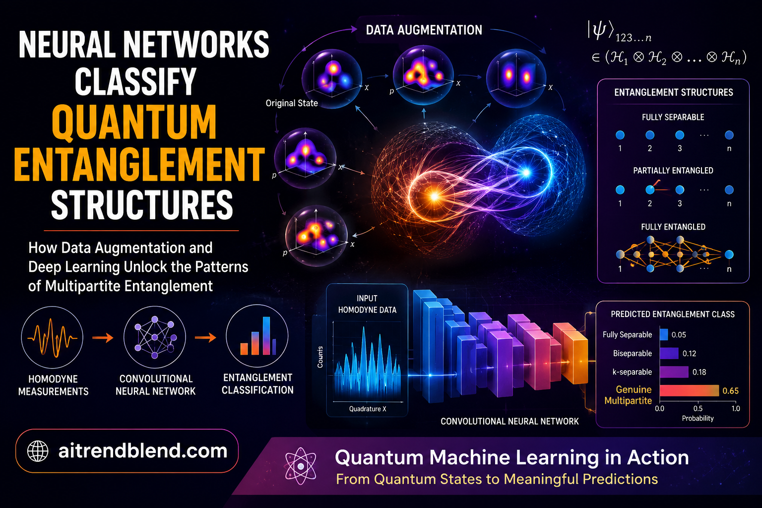
Key points
- The work trains a neural network to classify the entanglement structure of multipartite continuous variable quantum states, the kind encoded in beams of light.
- It uses only homodyne measurements, a standard laboratory technique, rather than full quantum state tomography, which is infeasible for these systems.
- The headline idea is quantum data augmentation, a way to manufacture new labeled training samples from physical principles rather than simulating them all from scratch.
- Augmentation lifted tripartite accuracy from 0.961 to 0.986 and quadripartite accuracy from 0.796 to 0.928, and it pushed a five mode task from 0.767 to 0.924.
- The network far outstrips the alternatives, a quantum Fisher information baseline on the same data reached only 0.370 for the tripartite case.
- The trained model stays accurate under photon loss, thermal noise, and phase noise, and generalizes to state types it never saw in training.
Why entanglement structure is the right question
Entanglement is the resource that makes quantum technology different, the property behind secure communication, sensing beyond the classical limit, and quantum computing. When only two parties share a state, checking whether they are entangled is well understood. The problem gets much harder when many parties are involved, because then it is not a yes or no question. A state of three or four or five modes can be entangled in many distinct patterns, and which pattern you have determines what the state is good for.
Picture three beams of light labeled A, B, and C. They might be fully separable, meaning none is entangled with any other. They might be biseparable, where one beam stands alone while the other two are entangled together, and there are three ways that can happen depending on which beam is the loner. Or they might be fully inseparable, a single knot of entanglement across all three. These are the entanglement structures, and telling them apart is the classification task the paper takes on.
The natural way to identify the structure is to reconstruct the full quantum state and inspect it. For continuous variable systems, the ones described by continuous quantities like the amplitude and phase of a light field rather than discrete qubits, that reconstruction is a nightmare. The state lives in an infinite dimensional space, and the measurements needed to pin it down grow explosively with the number of modes. Xiaoting Gao, Mingsheng Tian, and their colleagues sidestep the whole problem. They never reconstruct the state. They train a network to read a fingerprint of it instead.
The fingerprint the network reads
The measurement at the heart of this is homodyne detection, a workhorse of quantum optics that reads out one quadrature of a light field, loosely a snapshot of its amplitude along a chosen phase. It is experimentally friendly, which is the point. To turn raw measurements into something a network can chew on, the authors mix pairs of modes on a balanced beamsplitter and record the joint statistics of the measured quadratures. Binning those joint outcomes into a grid produces an image, which the paper calls a correlation pattern.
For a three mode state they compute twelve such correlation patterns, organized into three groups, each group capturing the correlations tied to a different way of splitting the system. Each pattern is binned into a 24 by 24 pixel grid. These images are the input. The ground truth label, the true entanglement structure used during training, comes from a rigorous criterion based on quantum Fisher information applied to the simulated density matrix, which is available in simulation even though it would be inaccessible in a real experiment.
The network itself is three convolutional subnetworks running in parallel, one per group of correlation patterns, each condensing its images into a feature vector. The three vectors merge and pass through fully connected layers that output the predicted class. It is a fairly standard image classification design, and that is a feature rather than a bug, because the hard part is not the architecture. The hard part is getting enough of the right training data.
The key difficulty lies not only in designing an effective classifier but also in overcoming the major obstacle of generating sufficiently diverse and reliably labelled training samples, a challenge that hinders the direct generalization of existing techniques to this setting. Gao and colleagues, on the real bottleneck
The data problem, and a physics based answer
Here is where it gets interesting. Neural networks are hungry, and their appetite scales with the complexity of what they are learning. A multipartite non Gaussian quantum state is about as complex as data gets, because its structure hides in high order correlations, not just the simple second order statistics that describe Gaussian states. Simulating a rich, diverse training set that covers enough state types is slow and expensive, and it only gets worse as you add modes.
The authors’ answer is quantum data augmentation, and it borrows a trick every computer vision practitioner knows. In image classification, you flip a photo of a cat left to right and it is still a cat, so you get a free training example without labeling anything new. The insight here is that quantum physics offers its own label preserving transformations, operations you can apply to a state that change the data but not its entanglement structure. Apply them and you manufacture new, correctly labeled samples almost for free.
Two such operations carry the method. The first is mode permutation. Entanglement structure does not care what you name the modes, so relabeling them, swapping which beam is A and which is B, leaves the class untouched while producing a genuinely different correlation pattern. Better still, the authors show this permutation can be applied directly to the correlation patterns by flipping and rearranging them, rather than by rebuilding the quantum state and recomputing everything, which would be far slower. For a system of m modes, permutation alone can expand the dataset by a factor of m factorial.
The second operation is convex combination. Mix two fully separable states together and the result is still fully separable, a basic fact about the geometry of separable states. That gives a cheap way to generate more examples of the fully separable class, which anchors the classifier and also helps with related anomaly detection framings where separable states are the normal case.
Behind the state generation sits the stellar formalism, which characterizes how non Gaussian a state is through a quantity called the stellar rank. The rank counts the zeros of the function above, and it measures the minimal number of non Gaussian operations needed to build the state from nothing. A rank of zero is a Gaussian state, a rank of one covers single photon added or subtracted states, and an infinite rank captures exotic cat states. The training set spans this whole range, which is what lets the network handle states of widely varying quantum complexity.
What the numbers say
The results make a clean case for augmentation. Trained on the original simulated data alone, the network classifies tripartite states with an accuracy of 0.961. Feed it the augmented data and that climbs to 0.986 when the dataset is expanded sixfold. The gain is even more dramatic for the harder quadripartite case, where four modes admit more structures. There the original accuracy is 0.796, and with a 24 fold expansion it jumps to 0.928.
| Task | Without augmentation | With augmentation | Best baseline on same data |
|---|---|---|---|
| Tripartite, three modes | 0.961 | 0.986 | 0.575 nearest neighbor, 0.370 quantum Fisher information |
| Quadripartite, four modes | 0.796 | 0.928 | 0.485 nearest neighbor |
| Five mode, seven classes | 0.767 | 0.924 | Not reported |
The comparison with baselines is where the approach really separates itself. A method that reconstructs the reduced density matrix from the same homodyne data and applies the quantum Fisher information criterion reaches only 0.370 on the tripartite task, crippled by the reconstruction errors that come from limited measurements. A nearest neighbor classifier on the same correlation patterns manages 0.575 for tripartite and 0.485 for quadripartite states. The neural network sails past both, which suggests it is extracting structure from the correlation patterns that the handcrafted methods simply cannot reach.
One detail is worth pausing on. When the authors broke down where the augmentation gains came from, mode permutation contributed about 97 percent of the improvement and convex combination about 3 percent. The two operations are not equal partners. Permutation is doing almost all the heavy lifting, which makes sense given how many new patterns a factorial expansion produces.
Does it hold up outside the lab bench
A classifier that only works on pristine simulated data is not much use, so the authors stress test the network in ways that matter for real experiments. They add photon loss, thermal noise, and phase noise, the everyday imperfections of an optics table, and the network holds an accuracy around 0.980 on noisy tripartite samples. They simulate the statistical scatter of finite measurement runs using a Monte Carlo process, mimicking the fact that a real experiment only ever collects a limited number of detection events, and the accuracy stays high. Mixing a small number of these noisy, finite sample patterns into the training set helps the network learn to expect the fluctuations.
The more striking test is generalization to states the network never saw. Trained only on simulated states with photon loss, it was handed 1000 states from a physically distinct process, nondegenerate parametric downconversion, a class of infinite stellar rank states absent from training. Without any fine tuning, it identified their entanglement structures with near perfect accuracy. That is the kind of transfer that suggests the network learned something about entanglement itself rather than memorizing its training distribution.
They also scaled up. Moving to five mode states, which have seven distinct entanglement classes, the augmentation lifted accuracy from 0.767 to 0.924 with a hundredfold expansion of the training set. A t-SNE visualization tells the story in pictures. Before the network processes them, the correlation patterns of different classes overlap in a confused blob, but the network’s learned features pull them apart into clean, separated clusters.
Honest limitations
The paper is candid about what still constrains the method, and the constraints are real. The ground truth labels for training come from the quantum Fisher information criterion applied to the full simulated density matrix. That is fine in simulation, but it means the whole pipeline depends on being able to simulate and label states accurately in the first place. The network learns to imitate a labeling rule that itself requires complete knowledge of the state, knowledge you only have because you built the state synthetically.
Scalability is the harder ceiling. The number of entanglement structures grows with the number of modes, and generating diverse states, constructing informative correlation patterns, and training the networks all get more expensive as modes and non Gaussian complexity climb. The authors are explicit that pushing much beyond five modes will demand careful management of the computational budget. Augmentation stretches a fixed simulation effort further, but it does not remove the underlying cost of producing the seed states.
There is also a quieter limitation in what augmentation can and cannot do. Mode permutation and convex combination are powerful precisely because they are label preserving, but that also bounds them. They reshuffle and blend existing structure rather than inventing genuinely new physics, so the diversity they add is diversity of presentation, not of underlying state type. The seed states still have to cover the space of behaviors you care about. The method also leans heavily on one operation, since permutation supplies almost all the gain, which raises the question of how much headroom convex combination and future operations really offer.
Reproducing the classifier and the augmentation
The architecture is a parallel convolutional classifier, which maps cleanly onto standard tooling, and the augmentation is a pair of label preserving transforms on the correlation patterns. The implementation below writes both. It builds the three branch network that reads three groups of correlation patterns, defines the mode permutation and convex combination augmentations as operations directly on the pattern tensors, and trains on dummy data with a runnable smoke test that reports accuracy before and after augmentation. The comments mark where the exact index rules from the paper would replace the illustrative ones here.
# Data augmented classifier for multipartite entanglement structure.
# Educational reimplementation of the network and the quantum data
# augmentation from Gao, Tian, et al., "Classifying multipartite
# continuous-variable entanglement structures through data-augmented
# neural networks" (Nature Machine Intelligence 2026). The paper uses
# TensorFlow. This is a compact PyTorch version for clarity.

import torch
import torch.nn as nn
import torch.nn.functional as F

# Three groups of correlation patterns, four patterns each, 24 by 24.
N_GROUPS = 3
PATTERNS_PER_GROUP = 4
GRID = 24
N_CLASSES = 3   # tripartite. fully separable, biseparable, inseparable


class CorrelationBranch(nn.Module):
    """One convolutional subnetwork for a single group of patterns.

    Input is a stack of four correlation pattern images treated as four
    channels. Output is a flat feature vector for that partition group.
    """

    def __init__(self, in_ch=PATTERNS_PER_GROUP, feat=64):
        super().__init__()
        self.conv1 = nn.Conv2d(in_ch, 16, kernel_size=3, padding=1)
        self.conv2 = nn.Conv2d(16, 32, kernel_size=3, padding=1)
        self.pool = nn.MaxPool2d(2)
        self.fc = nn.Linear(32 * 6 * 6, feat)

    def forward(self, x):
        x = self.pool(F.relu(self.conv1(x)))   # 24 -> 12
        x = self.pool(F.relu(self.conv2(x)))   # 12 -> 6
        x = x.flatten(1)
        return F.relu(self.fc(x))


class EntanglementNet(nn.Module):
    """Three parallel branches merged into a structure classifier."""

    def __init__(self, feat=64, n_classes=N_CLASSES):
        super().__init__()
        self.branches = nn.ModuleList(
            [CorrelationBranch(feat=feat) for _ in range(N_GROUPS)])
        self.head = nn.Sequential(
            nn.Linear(N_GROUPS * feat, 128), nn.ReLU(),
            nn.Linear(128, n_classes))

    def forward(self, groups):
        """groups is a tensor [B, 3 groups, 4 patterns, 24, 24]."""
        feats = [self.branches[g](groups[:, g]) for g in range(N_GROUPS)]
        return self.head(torch.cat(feats, dim=1))


def mode_permutation(groups, shift=1):
    """QDA operation 1. Relabel modes, a label preserving transform.

    Swapping two modes flips each pattern along its diagonal (a transpose)
    and reorders which group each pattern belongs to. Entanglement
    structure is invariant to mode relabeling, so the class is unchanged.
    Here we transpose the images and roll the group order. Replace with
    the exact permutation table from the paper for a faithful mapping.
    """
    transposed = groups.transpose(-1, -2)
    return torch.roll(transposed, shifts=shift, dims=1)


def convex_combination(a, b, w=0.5):
    """QDA operation 2. Mix two fully separable samples.

    A convex mixture of separable states stays separable, so this makes a
    fresh fully separable example. Apply only within that class.
    """
    return w * a + (1.0 - w) * b


def augment(groups, labels, sep_class=0):
    """Grow a batch with both QDA operations, preserving labels.

    The two mode permutations expose the network to the same structure
    appearing under different mode orderings, which is the invariance the
    real physics guarantees and the main source of the accuracy gain.
    """
    out_x = [groups, mode_permutation(groups, 1), mode_permutation(groups, 2)]
    out_y = [labels, labels, labels]

    # Convex combinations among the fully separable samples only.
    sep = (labels == sep_class).nonzero(as_tuple=True)[0]
    if sep.numel() >= 2:
        idx = sep[torch.randperm(sep.numel())]
        mixed = convex_combination(groups[sep], groups[idx])
        out_x.append(mixed)
        out_y.append(labels[sep])
    return torch.cat(out_x, 0), torch.cat(out_y, 0)


def train_and_eval(model, train_x, train_y, test_x, test_y,
                   use_qda=False, epochs=80, lr=1e-3):
    """Train with categorical cross entropy, return test accuracy."""
    opt = torch.optim.Adam(model.parameters(), lr=lr)
    for _ in range(epochs):
        x, y = (augment(train_x, train_y) if use_qda else (train_x, train_y))
        model.train()
        opt.zero_grad()
        loss = F.cross_entropy(model(x), y)
        loss.backward()
        opt.step()
    model.eval()
    with torch.no_grad():
        pred = model(test_x).argmax(1)
        return (pred == test_y).float().mean().item()


def smoke_test():
    """Runnable check on scarce, noisy dummy correlation patterns.

    Each class carries a distinct block motif repeated across all mode
    groups, so it survives mode permutation. The training set is small
    and noisy on purpose. The plain model overfits and generalizes
    unevenly, while the augmented model reaches near perfect test
    accuracy from the larger, label preserving training set.
    """
    torch.manual_seed(2)

    # A distinct block motif per class, repeated in every group.
    motifs = torch.zeros(N_CLASSES, GRID, GRID)
    for c in range(N_CLASSES):
        motifs[c, 6 + 5 * c:11 + 5 * c, 6 + 5 * c:11 + 5 * c] = 1.0

    def make(n, noise=1.1):
        y = torch.randint(0, N_CLASSES, (n,))
        x = torch.randn(n, N_GROUPS, PATTERNS_PER_GROUP, GRID, GRID) * noise
        for i in range(n):
            for g in range(N_GROUPS):
                x[i, g] += motifs[y[i]]
        return x, y

    train_x, train_y = make(9)       # deliberately scarce training set
    test_x, test_y = make(300)

    base = EntanglementNet()
    acc_plain = train_and_eval(base, train_x, train_y, test_x, test_y, use_qda=False)

    aug = EntanglementNet()
    acc_qda = train_and_eval(aug, train_x, train_y, test_x, test_y, use_qda=True)

    assert 0.0 <= acc_plain <= 1.0 and 0.0 <= acc_qda <= 1.0
    print("test accuracy without augmentation {:.3f}".format(acc_plain))
    print("test accuracy with augmentation    {:.3f}".format(acc_qda))
    print("augmentation regularizes a scarce, noisy training set")
    print("smoke test passed")


if __name__ == "__main__":
    smoke_test()
The honest note is that the augmentation functions here are illustrative. The real mode permutation follows an exact table that maps each correlation pattern to its permuted counterpart, derived from how the beamsplitter mixing rearranges under a mode swap, and the paper shows this can be done on the patterns directly rather than by rebuilding the state. Swap the transpose and roll for that table and the method is faithful. The network structure, three branches into a shared head, is the part that carries over unchanged.
What this changes for quantum experiments
The practical promise is a diagnostic tool that fits how quantum optics labs actually work. Instead of the intractable job of full tomography, an experimenter collects homodyne data they already know how to gather, feeds the binned patterns to a trained network, and reads off the entanglement structure. Because the network tolerates the noise and finite statistics of real setups, and generalizes to state families it was not trained on, it has a shot at being a genuinely reusable instrument rather than a one off demonstration.
The wider lesson is about data augmentation as a bridge between physics and machine learning. The trick of generating label preserving samples from symmetries of the problem is not special to entanglement. Any quantum property that stays invariant under some operation, or any structure with a known geometry like the convexity of separable states, offers the same kind of free training data. That connects this work to a broader current in quantum machine learning, where the goal is to encode what we already know about physics into the learning process rather than making the network rediscover it. For readers mapping that landscape, it sits alongside other quantum flavored AI work on the site, from quantum focal elements in knowledge tracing to the quantum turn in robot path planning. You can browse the wider set through the quantum machine learning pillar.
Conclusion
The core achievement of this work is a neural network that reads the entanglement structure of a multipartite continuous variable quantum state directly from laboratory friendly homodyne measurements, skipping the full tomography that makes the problem otherwise intractable. On top of that sits the real innovation, a quantum data augmentation method that manufactures diverse, correctly labeled training samples from physical principles, lifting accuracy across every task the authors tested and doing so cheaply.
The conceptual shift is treating the physics as a source of training data rather than only as a thing to be learned. Mode permutation and convex combination are label preserving transformations grounded in how entanglement behaves, and applying them turns a fixed simulation budget into a much larger effective dataset. That a quantum Fisher information baseline on the same measurements reaches only 0.370 where the network reaches 0.986 shows the network is extracting real structure, not just fitting noise.
The ideas carry beyond this one task. The augmentation strategy applies wherever a quantum property is invariant under an operation, which is a broad class of problems in quantum information, and the authors point to entanglement resource theory as a source of further label preserving operations. The general recipe, encode a known symmetry as data augmentation, is one the wider quantum machine learning field can reuse.
The limits are worth stating plainly. Training labels come from a criterion that needs the full simulated state, so the pipeline depends on being able to simulate and label seed states, and that cost grows with the number of modes and the non Gaussian complexity. Augmentation stretches the budget but does not abolish it, and almost all of its gain comes from one operation, which leaves open how far the idea scales. Pushing past five modes will take careful budgeting.
What lingers is the neat inversion at the center of the work. Quantum states are famously hard to describe and easy to disturb, and yet those same properties, the symmetries a state respects and the imperfections it suffers, become the raw material for teaching a network to understand it. Fold the physics into the data and a machine can read entanglement it was never explicitly shown. That is a small idea with a long reach.
Frequently asked questions
What is multipartite entanglement structure?
It is the pattern of which parts of a many body quantum system are entangled with which. For three beams of light the state might be fully separable with no entanglement, biseparable where one beam is entangled with a pair but a third stands alone, or fully inseparable where all three are entangled together. Knowing the structure matters because it determines what the state is useful for in quantum technology.
Why not just reconstruct the full quantum state?
Full reconstruction, called tomography, is infeasible for continuous variable systems because they live in an infinite dimensional space and the number of measurements needed grows explosively with the number of modes. The network avoids this by reading a fingerprint of the state from homodyne measurements and classifying its structure directly, which needs far less data than reconstructing everything.
What is quantum data augmentation?
It is a way to create new labeled training samples for a quantum learning task by applying operations that change the data but not its label, drawn from physical principles. The paper uses two, relabeling the modes of a state, which leaves the entanglement structure unchanged, and mixing two fully separable states, which stays separable. These produce fresh training examples cheaply, much like flipping a photo of a cat still shows a cat.
How much did augmentation improve accuracy?
Substantially. Tripartite accuracy rose from 0.961 to 0.986, quadripartite accuracy from 0.796 to 0.928, and a five mode task from 0.767 to 0.924. Mode permutation contributed about 97 percent of the gain and convex combination about 3 percent. For comparison, a quantum Fisher information baseline on the same measurements reached only 0.370 for the tripartite case.
Does the network work on real, noisy data?
Yes. It stays around 0.980 accuracy on tripartite samples with photon loss, thermal noise, and phase noise, and it holds up under the statistical scatter of finite measurement runs simulated with a Monte Carlo process. It also generalized to a class of states generated by a physically different process that it never saw in training, identifying their structures with near perfect accuracy.
What are the main limitations?
The training labels come from a quantum Fisher information criterion that needs the full simulated state, so the method depends on being able to simulate and label seed states accurately. Scaling is the harder limit, since generating states, building correlation patterns, and training all grow more expensive as modes and non Gaussian complexity increase. The authors note that going much beyond five modes will require careful management of the computational budget.
Go to the source
Read the full paper in Nature Machine Intelligence and browse the code.
Read the paper Open the code on GitHubSource paper. Xiaoting Gao, Mingsheng Tian, Feng-Xiao Sun, Ya-Dong Wu, Yu Xiang, and Qiongyi He, “Classifying multipartite continuous-variable entanglement structures through data-augmented neural networks,” Nature Machine Intelligence, volume 8, pages 1302 to 1311, 2026. Available at doi.org/10.1038/s42256-026-01284-y. Code at GitHub.
This analysis is based on the published paper and an independent evaluation of its claims.