
You decide you want a hammer. Within a second your mind has sketched a rough plan. Walk to the garage, open the third drawer, and if it is not there, check the shed. You did not search over every possible action in the house, and you did not train on a million labelled examples. You imagined a route to the goal and started moving.
Your brain did all of that on about twenty watts, less than a dim bulb. A team from Tsinghua University, Graz University of Technology, and the National Research Council in Rome has built a small neural model that plans the same way, and the surprising claim is that it needs neither a deep network nor a large language model to do it.
Key points
- The model, called GCML, learns a cognitive map from grid cell activity and then imagines routes to a goal by sampling trajectories, the same trick the rodent brain appears to use during hippocampal replay.
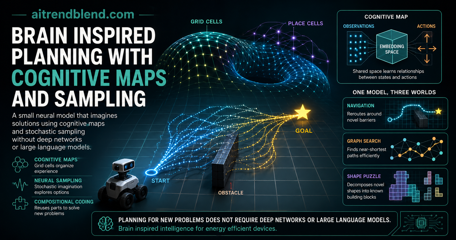
- Three brain ingredients do the work. A cognitive map for organizing experience, stochastic sampling for exploring options, and compositional coding for reusing parts across new problems.
- It planned across three very different worlds. Two dimensional navigation with novel barriers, an abstract graph search, and an NP hard puzzle of decomposing shapes into building blocks it had never seen.
- On the shape puzzle it beat a deep reinforcement learning agent and a model predictive control baseline, reaching near perfect success with about twenty samples while using only simple local learning rules.
- The learning is self supervised and local, so it fits energy efficient neuromorphic chips. The headline is blunt. Planning for genuinely new problems does not require deep networks or large language models.
The energy gap that started the whole thing
Modern artificial intelligence is getting smarter and hungrier at the same time. Training a frontier model burns through power and hardware at a scale that would have looked absurd a decade ago. The brain sits on the other side of that gap. It runs on the power of a night light, it learns while it works rather than in a separate training phase, and it adjusts the moment the world changes.
That contrast is the motivation behind this paper. The authors, led by Wolfgang Maass in Graz, ask a pointed question. What data structures and learning rules let a brain plan so cheaply, and can those be ported into a device? They zero in on one capacity that sits at the heart of intelligence, the ability to solve a new problem, including one whose states were never seen before, and they try to reproduce it with tools a brain plausibly uses rather than with the machinery of deep learning.
Three tools carry the argument. Cognitive maps, which organize experience into a structure that relates states and actions. Stochastic computing, meaning the brain samples possibilities rather than computing one deterministic answer. And compositional coding, the habit of describing new things as fresh combinations of familiar parts. The contribution is a single transparent model that welds all three together, named the Generative Cognitive Map Learner, or GCML.
What a cognitive map actually is here
Start with the brain part, because the model borrows its bones. Deep in the entorhinal cortex sit grid cells, neurons that fire in a repeating triangular pattern as an animal moves through space. Together they act like a coordinate system that the brain keeps updated through path integration, quietly adding up each small movement to track where the body is. The authors model roughly one thousand such cells, and a striking geometric fact falls out. The collective activity of a grid cell population lives on the surface of a torus, and a large enough patch of that torus is nearly flat, which is exactly what you want if you are mapping a flat room.
On top of the grid cells sit place cells, which fire at specific locations, and a set of action neurons that encode movement directions. The model learns two embeddings that tie these together. One matrix embeds observations into a shared high dimensional space, and another embeds actions into the same space. The point of sharing the space is that the geometry of the map then captures the relationships between where you are and what you can do, which is the raw material for planning.
Crucially, the authors show that the same idea works for problems that have nothing to do with physical space. A concept space, a graph of abstract states, a puzzle of shapes, all of them can be given a cognitive map of the same kind, as long as the map has enough dimensions to hold the structure. That generality is what lets one model plan a walk to the kitchen and decompose an abstract silhouette with the same machinery. For a very different take on turning a problem into a graph a machine can plan over, our piece on goal oriented graphs for language model planning arrives at planning from the opposite direction, leaning on a large model rather than avoiding one.
Learning the map, then imagining with it
Two models sit at the core, and the names matter. The first is the CML, a deterministic learner that watches the world, predicts what it will see next after an action, and adjusts its embeddings whenever the prediction misses. This is predictive coding in plain clothes. It only needs a local rule, a small update that compares the prediction to the outcome and nudges the weights, which is the kind of thing a synapse can actually do without any global backpropagation.
The second model is the star, the GCML, a generative twist on the first. It adds two things. It learns an inverse model, a weight matrix that reads the difference between where you are and where you want to be and turns that gap into an action. And it injects noise into that action choice, which converts a rigid controller into something that samples. Give it a goal and it does not compute one path. It imagines many, and because the noise is tunable, you control how adventurous the imagination gets.
The bootstrapping loop
Here is the part that makes imagination possible without moving a muscle. Normally the model acts, the world hands back an observation, and the loop continues. During planning there is no world to answer, so the model answers itself. After choosing a virtual action, it predicts the next state with its own forward model and feeds that prediction back in as if it had really happened. Round and round this goes, and out comes an imagined sequence of steps that walks from the start toward the goal, entirely inside the network.
The model plans by talking to itself. It proposes an action, predicts the result, believes its own prediction, and repeats. The noise sprinkled into each choice is what turns a single rigid plan into a spread of plausible ones a downstream circuit can pick from.
The equations behind the loop
The forward model is a linear prediction. The estimated next state is the current state plus the effect of the chosen action, and learning drives that estimate toward the true embedding of the next observation.
The inverse model turns a goal gap into a drive. It multiplies the difference between the goal state and the current state by the learned matrix, adds noise, and scales the result into an action.
Every matrix here is trained by a local rule. The inverse model, for instance, learns by a simple Hebbian product of the action taken and the state change it caused.
One elegant consequence deserves a pause. That inverse matrix behaves like a value function from reinforcement learning, scoring how useful each action is for reaching the goal. But unlike a reinforcement learning policy, it is not tied to one goal. It works for any goal you hand it, because it reads the gap rather than memorizing a route. Swap the goal and nothing needs retraining. Readers who have followed the pain of training reinforcement agents on neuromorphic hardware will appreciate why that matters, a theme our review of spiking deep reinforcement learning digs into from the hardware side.
Three worlds, one model
The proof is in the range. The authors turned the same machine loose on three problems that share almost nothing on the surface.
Walking, and rerouting around a new wall
The first world is ordinary two dimensional navigation. The model learns a spatial map by wandering a room, then imagines trajectories to a goal. What makes this more than a toy is how closely the imagined paths match real recordings from the rodent hippocampus. When the animal plans, its place cells replay routes to remembered goals, and those replays are diverse and rarely straight. The model reproduces that texture, including the behaviour that first puzzled neuroscientists, the ability to reroute around a barrier that was dropped into the environment after learning. Obstacles enter the model as repulsive forces, and the imagined path bends away from a wall even when that means briefly moving away from the goal before curving back.
Searching an abstract graph
The second world drops space entirely. Take a random graph of thirty two nodes, call the nodes states and the edges actions, and ask for a short path from a start to a distant goal. This is the classic problem of finding several near shortest routes, and exact algorithms solve it perfectly. The interesting result is that the GCML does not return one answer. It returns a menu of good ones, all clustered near the shortest possible length, and it does so with a self correcting homing instinct. Even when a bad first move gets sampled, the later steps drift back toward the goal on average. Turn the noise up and the menu grows more varied, which is useful when you want options rather than a single optimum.
Decomposing shapes it never saw
The third world is the hardest and the most convincing. Picture a black silhouette on a grid and a set of building blocks, small tile shapes. The task is to decompose the silhouette into those blocks with no gaps or overlaps. This is a genuinely hard problem, formally NP hard, and it was recently used to study compositional thinking in the human brain. The model was trained on decompositions of shapes made from five blocks, then tested on shapes it had never encountered, including harder ones built from eight blocks. It generalized, imagining valid decompositions of novel silhouettes through the same goal directed sampling.
The same cognitive map that walked the model to a kitchen also solved an abstract NP hard puzzle whose states were never visited during training. Compositional coding is what let it treat a new shape as a fresh arrangement of familiar parts.
How it stacks up against the usual suspects
A brain inspired story is charming, but the paper earns its place by measuring the model against methods people actually use.
| Problem | Compared against | How the GCML did |
|---|---|---|
| Two dimensional navigation | Rodent hippocampal recordings | Reproduced goal directed replay and rerouted around a barrier added after learning |
| Near shortest paths, graphs of 32 to 160 nodes | K*, mA*, and BELA* exact algorithms | Close to optimal path lengths, far fewer nodes visited, and almost no cost to replan when the goal moved |
| Silhouette decomposition, an NP hard puzzle | Deep reinforcement learning (D3QN), model predictive control, random | Highest success rate with about twenty samples, using only simple local updates |
Two comparisons stand out. Against the exact path finding algorithms, the GCML is not trying to win on optimality, and it gives up a little length on the largest graphs. What it wins on is effort. It explores far fewer nodes because the learned map points it in roughly the right direction from the start, and when the goal changes it pays almost nothing to replan, since the map already holds a sense of direction to anywhere. The classical methods have to search the graph again. If you want the fuller landscape of how path planning has evolved from these classical searches toward learned and even quantum methods, our review of robot path planning maps the territory.
Against the learning based methods on the shape puzzle, the GCML came out ahead of both a dueling double deep Q network and a model predictive control planner across almost every sample budget. The reinforcement agent needs backpropagation, which is awkward on neuromorphic hardware and unstable when the reward signal is sparse. The control planner pays a fresh optimization cost at every single step. The GCML leans on its learned map and simple local updates, which is why it stays cheap. That comparison with model predictive control is worth holding next to a working robotics example, such as the multi drone search system that uses exactly that style of control in the field.
A core feature of brain intelligence, the capacity to generate solutions to problems that were never encountered before, does not require deep neural networks or large language models, and can be implemented in energy efficient edge devices. Lin and colleagues, Nature Machine Intelligence, 2026
Why the hardware angle is the real prize
The most consequential part of this work is easy to skim past. Every learning rule in the GCML is local and self supervised. A weight changes based only on signals available right where it sits, the activity on either side of the connection and a local error, with no need to ship gradients backward through the whole network. That is precisely the property that neuromorphic and in memory computing hardware wants, because those chips struggle with the global bookkeeping that backpropagation demands.
The action selection is friendly too. Choosing the next move reduces to a winner take all over the candidate actions, which a small circuit of neurons with lateral inhibition can approximate, and the delay does not grow with the size of the environment. Put together, the model sketches a path toward edge devices that can imagine and plan on a tiny power budget rather than calling home to a data center. In a field that keeps solving problems by making models bigger, a result that solves them by making the algorithm more brain like is a refreshing turn.
Where it falls short
The authors are careful about the limits, and a fair reading has to sit with them.
This is a heuristic online method, not an optimal solver. It generates a promising first step from a sense of direction rather than proving that a plan is best, so on hard instances a more deliberate search will still find better solutions. On the largest graphs its path lengths degrade slightly, and for tricky obstacles such as a U shaped trap the model needs higher noise to escape, which can make it less stable. Imagination that samples widely is powerful and also messy.
There is a modelling simplification worth naming. The generative behaviour comes from adding Gaussian noise to a deterministic inverse model, which amounts to assuming a fixed uncertainty during sampling rather than learning the true uncertainty of the world. The authors flag this openly and point to richer probabilistic approaches as future work. A model that learned its own uncertainty, rather than having it dialed in, would connect more cleanly to the Bayesian view of planning as inference.
And the scope, while broad, is still a set of curated demonstrations. Two dimensional maps suffice for navigation, but the authors are explicit that non planar graphs and compositional puzzles need higher dimensional maps, and scaling those maps to the messiness of a real robot or a real language task is unproven. A plausible imagined plan is also not a guaranteed one. The model can dream a route that a real body could not execute, which is why the affordance gating that blocks infeasible actions is doing quiet but essential work.
A reference implementation
The code below is a compact, runnable version of the core idea. It learns the forward embeddings and the inverse model from random exploration of a small grid, using only local update rules, then imagines a goal directed path by running the bootstrapping loop with a little noise and a winner take all action choice. The authors full code and data are linked under the block.
# Generative Cognitive Map Learner, compact reference
# Learns forward embeddings Q and V and an inverse model W with local rules,
# then imagines a goal directed path by sampling, no backpropagation.

import numpy as np

rng = np.random.default_rng(0)

# A small 6 by 6 grid world. Observation is a one hot over the 36 cells.
GRID = 6
N_CELLS = GRID * GRID
N_STATE = 24          # dimension of the shared embedding space
ACTIONS = {0: (0, 1), 1: (0, -1), 2: (1, 0), 3: (-1, 0)}   # up down right left
N_ACT = len(ACTIONS)


def one_hot(idx, size):
    v = np.zeros(size)
    v[idx] = 1.0
    return v


def cell_id(x, y):
    return y * GRID + x


def step(x, y, a):
    # move if inside the grid, otherwise stay put
    dx, dy = ACTIONS[a]
    nx, ny = x + dx, y + dy
    if 0 <= nx < GRID and 0 <= ny < GRID:
        return nx, ny
    return x, y


# Embeddings and inverse model, initialised small and random.
Q = rng.normal(0, 0.1, size=(N_STATE, N_CELLS))    # observation embedding
V = rng.normal(0, 0.1, size=(N_STATE, N_ACT))      # action embedding
W = rng.normal(0, 0.01, size=(N_ACT, N_STATE))     # inverse model

eta_q = eta_v = 0.01
eta_w = 0.05


# 1. Learn from random exploration using only local delta and Hebbian rules.
def explore(steps=40000):
    global Q, V, W
    x, y = rng.integers(GRID), rng.integers(GRID)
    for _ in range(steps):
        a = rng.integers(N_ACT)
        o_t = one_hot(cell_id(x, y), N_CELLS)
        nx, ny = step(x, y, a)
        o_next = one_hot(cell_id(nx, ny), N_CELLS)

        s_t = Q @ o_t
        s_next = Q @ o_next
        a_vec = one_hot(a, N_ACT)

        # forward prediction and its error
        s_hat = Q @ o_t + V @ a_vec
        err = s_next - s_hat
        V += eta_v * np.outer(err, a_vec)              # delta rule for V
        Q += eta_q * np.outer(err, o_t)                # delta rule for Q

        # inverse model, Hebbian on action and state change
        W += eta_w * np.outer(a_vec, s_next - s_t)

        x, y = nx, ny


# 2. Imagine a goal directed path with the bootstrapping loop.
def imagine(start, goal, noise=0.4, max_steps=40):
    sx, sy = start
    gx, gy = goal
    s_hat = Q @ one_hot(cell_id(sx, sy), N_CELLS)
    s_goal = Q @ one_hot(cell_id(gx, gy), N_CELLS)
    path = [(sx, sy)]
    x, y = sx, sy
    for _ in range(max_steps):
        u = W @ (s_goal - s_hat) + rng.normal(0, noise, size=N_ACT)   # utility plus noise
        a = int(np.argmax(u))                                        # winner take all
        x, y = step(x, y, a)
        path.append((x, y))
        s_hat = s_hat + V @ one_hot(a, N_ACT)                        # believe own prediction
        if (x, y) == (gx, gy):
            break
    return path


if __name__ == "__main__":
    explore()
    for trial in range(3):
        p = imagine(start=(0, 0), goal=(5, 5))
        reached = p[-1] == (5, 5)
        print(f"trial {trial + 1}  steps {len(p) - 1}  reached {reached}  path {p}")
Go to the source
Read the peer reviewed paper and run the authors own code and data.
Read the paper Code on GitHubConclusion
The core achievement here is a single small model that plans across three worlds with the same parts. It learns a cognitive map, samples imagined trajectories toward a goal, and reuses familiar building blocks to attack problems it has never seen. It reproduces the diverse, rerouting replay that neuroscientists record in the rodent brain, it returns a menu of near optimal routes on an abstract graph, and it solves an NP hard shape puzzle on shapes outside its training set. None of that leans on a deep network or a large language model.
The conceptual shift worth remembering is the marriage of three ingredients that are usually studied apart. A cognitive map gives the model a sense of direction to anywhere. Stochastic sampling turns that sense of direction into a spread of options rather than one brittle plan. Compositional coding lets the map describe a new problem as an arrangement of parts it already understands. Each alone is familiar. Bolted together with local learning rules, they produce something that looks a lot like intuition, the ability to take a sensible first step toward a goal without laboriously mapping out the whole solution first.
The approach travels because it is not really about hammers or hippocampi. The same recipe applies to any domain you can cast as a map of states and actions, from spatial navigation to abstract reasoning, provided the map has room for the structure. That transferability is arguably the larger contribution, since it hands a planning method to fields that never had a cognitive map of their own, all while keeping the compute small enough for an edge device.
The honest limits keep it grounded. This is a heuristic that generates a good first move, not a solver that guarantees the best plan. It leans on noise it does not learn, it degrades on the largest problems, and its demonstrations, while broad, are still curated rather than deployed in the wild. A plausible imagined plan is not a validated one, and the affordance gate that filters out impossible actions is doing quiet, essential work behind the scenes.
Future directions almost write themselves. Learn the uncertainty rather than dialing it in, which would connect the model to planning as probabilistic inference. Combine the low latency of this approach with the deeper search of model predictive control in a hybrid. Push the maps to higher dimensions and see whether the same trick scales to a real robot or a real reasoning task. If those steps hold up, the quiet promise of this paper, that a brain like algorithm can plan for genuinely new problems on twenty watts, becomes something you could hold in your hand.
Frequently asked questions
What is a cognitive map in this model?
It is a learned high dimensional space, built from grid cell activity, that places observations and actions together so their geometric relationships capture how states connect. The same kind of map works for physical space and for abstract problems.
How does the model plan without moving?
It uses a bootstrapping loop. After choosing a virtual action it predicts the resulting state with its own forward model, feeds that prediction back in as if it were real, and repeats, generating an imagined path from start to goal entirely inside the network.
Why does it not need a deep network or a large language model?
The planning comes from a learned cognitive map and simple local learning rules rather than from many stacked layers trained by backpropagation. The authors show this is enough to solve new problems, which is why it can run on energy efficient hardware.
How did it compare with reinforcement learning?
On an NP hard shape decomposition puzzle it beat a dueling double deep Q network and a model predictive control planner across most sample budgets, reaching near perfect success with about twenty samples while using only local updates.
What are the three brain ingredients it combines?
Cognitive maps for organizing experience, stochastic sampling for exploring many possible plans, and compositional coding for describing new problems as combinations of familiar parts. The model welds all three into one system.
Can the code and data be reproduced?
Yes. The authors released their code and data on GitHub and Zenodo under an open licence, so the navigation, graph search, and shape decomposition results can be reproduced and extended.