
- Graph neural networks
- Message passing
- Graph Laplacian
- Spectral filters
- GCN and GAT
- Oversmoothing
- PyTorch
A new paper lands in a citation database with a title, an abstract and a reference list. Nobody has labelled its field yet. A text classifier would read the abstract and guess. A graph neural network does something else. It also looks at the papers this one cites, and the papers those cite, and lets their topics pull on its prediction.
That idea sounds almost too simple to need mathematics. It turns out to rest on a surprising amount of it. There is linear algebra from spectral graph theory, a counting argument from a 1968 graph isomorphism test, a smoothing process that can erase what it was meant to share, and a bottleneck that no amount of depth can fix. This piece works through each of them with one small graph and a handful of derivations.
Key points
- A graph layer must give the same answer when nodes are renumbered, which forces it to aggregate neighbours with symmetric operations such as a sum or mean.
- The graph Laplacian turns smoothness into a number, the Dirichlet energy, and its eigenvectors give graphs their own version of a Fourier basis.
- The GCN layer is a first order Chebyshev filter with a renormalization trick, and it acts as a low pass filter that keeps smooth signals and suppresses sharp ones.
- Message passing networks can never distinguish more graphs than the Weisfeiler and Leman test, and only sum style aggregation reaches that ceiling.
- Deep stacks shrink the Dirichlet energy geometrically, which is oversmoothing, while tree like bottlenecks limit how much distant information can arrive, which is oversquashing.
- A PyTorch file at the end implements GCN, GAT, GraphSAGE, GIN, APPNP and EGNN and checks eleven of the identities numerically.
Why Graphs Break Ordinary Neural Networks
An image has a grid. Pixel (3, 4) always sits to the left of pixel (3, 5), and a convolution kernel can rely on that. A sentence has an order. A graph has neither. A molecule, a road network or a social network is a set of nodes and a set of edges, and the numbering of the nodes is an accident of how the file was written.
Write the graph as an adjacency matrix \( A \in \{0,1\}^{N \times N} \) with node features \( X \in \mathbb{R}^{N \times d} \). Renumbering the nodes with a permutation matrix \( P \) gives \( PX \) and \( PAP^{\top} \), which describe exactly the same graph. So any sensible model must respect that symmetry.
A graph level prediction, such as whether a molecule is toxic, should not change at all. A node level prediction, such as the field of each paper, should be shuffled in exactly the same way as the nodes. Michael Bronstein, Joan Bruna, Taco Cohen and Petar Veličković built a whole framework on this observation in their geometric deep learning monograph. Convolutions respect translations, recurrent networks respect time, and graph networks respect permutations.
A plain multilayer perceptron applied to the flattened adjacency matrix fails the test immediately. Relabel two nodes and every input position changes. The earliest graph neural network, introduced by Franco Scarselli, Marco Gori and colleagues in The Graph Neural Network Model in 2009, solved this by letting each node update its state from its neighbours until the states reached a fixed point. Almost everything since has kept the neighbourhood idea and dropped the fixed point.
The site’s graph neural networks hub collects every paper analysis we have published on the topic. This article is the mathematical background those pieces assume.
The Running Example
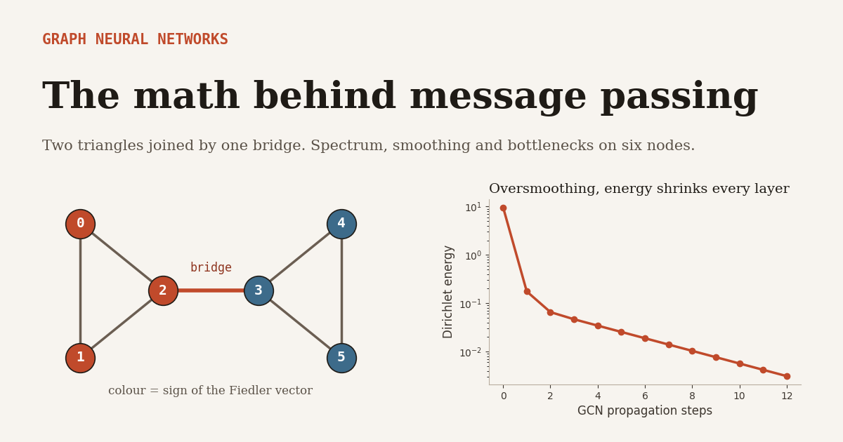
Everything below uses one graph with six nodes. Nodes 0, 1 and 2 form a triangle. Nodes 3, 4 and 5 form a second triangle. A single bridge edge connects node 2 to node 3. It is small enough to compute by hand, and it happens to show every phenomenon in this article, communities, smoothing and a bottleneck.
Nodes 0, 1, 4 and 5 have degree 2. The two bridge nodes have degree 3. Keep that asymmetry in mind, because the normalization in a GCN is entirely about degrees.
The Message Passing Template
Justin Gilmer, Samuel Schoenholz, Patrick Riley, Oriol Vinyals and George Dahl unified a zoo of graph models in Neural Message Passing for Quantum Chemistry in 2017. Their template has two steps per layer. Every node collects messages from its neighbours, then updates its own state.
The message function \( M_t \) and update function \( U_t \) are small neural networks shared across all nodes. After T layers a readout pools node states into a single vector for graph level tasks.
Why is this permutation equivariant? Because the sum over a neighbourhood does not care in what order the neighbours are listed. Relabel the nodes and each node receives the same multiset of messages as before, only under a new name. The same argument works for a mean or a maximum. It fails for anything that depends on order, such as feeding neighbours into a recurrent network, which is why GraphSAGE had to shuffle neighbours randomly when it tried an LSTM aggregator.
Two consequences follow from the template directly. After t layers, a node’s state depends only on nodes within t hops, so depth sets the receptive field. And the parameters do not depend on the number of nodes, so the same model runs on a molecule with twelve atoms and a citation graph with twenty thousand papers.
The Laplacian and What Smoothness Means on a Graph
Before the practical layers make sense, one object needs an introduction. The combinatorial graph Laplacian is the degree matrix minus the adjacency matrix.
Its power comes from one identity. For any signal \( x \) that assigns a number to each node, the quadratic form of \( L \) adds up squared differences across edges.
To see it, expand \( x^{\top}Dx – x^{\top}Ax = \sum_i d_i x_i^2 – \sum_{i,j} A_{ij} x_i x_j \). Every edge contributes \( x_i^2 + x_j^2 \) to the first sum and \( 2x_ix_j \) to the second, which is exactly \( (x_i – x_j)^2 \). This quantity is called the Dirichlet energy. It is zero when the signal is constant across every connected component and large when neighbours disagree. It is the graph version of the integral of a squared gradient, and it will be the main tool for measuring oversmoothing later.
The Laplacian is symmetric and positive semidefinite, so it has an orthonormal eigenbasis \( L = U \Lambda U^{\top} \) with eigenvalues \( 0 = \lambda_1 \le \lambda_2 \le \dots \le \lambda_N \). Each eigenvector is a signal on the nodes, and its eigenvalue is its own Dirichlet energy. Small eigenvalues belong to smooth signals. Large eigenvalues belong to signals that flip sign across many edges. That is exactly the relationship between frequency and oscillation in ordinary Fourier analysis.
For the running example, the normalized Laplacian has eigenvalues 0, 0.205, 1.167, 1.5, 1.5 and 1.629. The second eigenvector, called the Fiedler vector, has entries of about 0.45, 0.45 and 0.32 on the first triangle and the same values with a negative sign on the second. Its sign splits the graph exactly at the bridge. That is spectral clustering in one line, and it is why the feature image colours the two triangles differently.
The eigenvalues of \( L_{\text{sym}} \) always lie between 0 and 2. The value 2 is reached only by bipartite components. Both facts matter shortly.
The Spectral Road to Graph Convolution
With a Fourier basis in hand, convolution follows from the convolution theorem. Transform the signal into the spectral domain with \( \hat{x} = U^{\top}x \), multiply each frequency by a filter coefficient, and transform back.
Joan Bruna, Wojciech Zaremba, Arthur Szlam and Yann LeCun trained filters of this form directly in Spectral Networks and Locally Connected Networks on Graphs in 2014, with one free parameter per eigenvalue. Three problems made the approach impractical. The eigendecomposition costs \( O(N^3) \), applying \( U \) costs \( O(N^2) \) per signal, and a filter learned on one graph means nothing on another graph with a different eigenbasis. Worse, a filter with arbitrary coefficients is not spatially local. Every node can influence every other node in one layer.
Chebyshev polynomials make filters local
Michaël Defferrard, Xavier Bresson and Pierre Vandergheynst fixed all three problems in Convolutional Neural Networks on Graphs with Fast Localized Spectral Filtering in 2016. Their idea was to restrict the filter to a polynomial of the eigenvalues. A polynomial of \( \Lambda \) sandwiched between \( U \) and \( U^{\top} \) is simply the same polynomial of \( L \), so the eigenvectors are never needed.
The rescaled Laplacian \( \hat{L} \) has eigenvalues in \( [-1, 1] \), the natural domain of Chebyshev polynomials, and the recurrence means each extra order costs one sparse matrix product. Locality falls out for free. The matrix \( L^k \) has a nonzero entry \( (i,j) \) only if nodes i and j are within k hops, so an order K filter is exactly K hop localized. The code at the end confirms that the Chebyshev recurrence and the explicit spectral formula give identical outputs on the running example.
From ChebNet to GCN in three approximations
Thomas Kipf and Max Welling simplified ChebNet into the layer that became the default for years, in their GCN paper at ICLR 2017. The derivation takes three steps, and each one is a deliberate trade.
First, keep only K equal to 1, so each layer looks one hop away and depth provides the rest. Second, approximate \( \lambda_{\max} \approx 2 \), the upper bound for the normalized Laplacian. The rescaled Laplacian becomes \( L_{\text{sym}} – I = -D^{-1/2}AD^{-1/2} \) and the filter reduces to two terms.
Third, tie the two parameters together with \( \theta = \theta_0′ = -\theta_1′ \), which halves the parameter count and acts as a regularizer.
There is a problem hiding in Equation 8. The eigenvalues of \( D^{-1/2}AD^{-1/2} \) lie in \( [-1, 1] \), so the eigenvalues of \( I + D^{-1/2}AD^{-1/2} \) lie in \( [0, 2] \). Stack twenty such layers and any component with eigenvalue near 2 grows like \( 2^{20} \), while the gradient on any component near 0 vanishes. Kipf and Welling fixed this with what they called the renormalization trick. Add self loops first and normalize afterwards.
Call the propagation matrix \( P = \tilde{D}^{-1/2}\tilde{A}\tilde{D}^{-1/2} \). Its largest eigenvalue is exactly 1, and the self loops push the smallest eigenvalue strictly above \( -1 \). On the running example the eigenvalues of \( P \) are 1, 0.860, 0.167, 0, 0 and \( -0.194 \). Nothing grows, and the negative end is well away from the oscillating value of \( -1 \) that would make repeated application flip signs.
The symmetric normalization also has a clean reading in the node domain. Entry \( P_{ij} = 1/\sqrt{\tilde{d}_i \tilde{d}_j} \) for neighbours, so a message from a high degree hub is damped, and so is the total a hub receives. In the running example, node 0 gives weight 1/3 to itself and to node 1, but only about 0.289 to node 2, because node 2 is a bridge with a higher degree.
The GCN layer is not an arbitrary design. It is a one hop Chebyshev filter with two approximations and one stability fix. Every term in Equation 9 traces back to a spectral argument, which is also why its behaviour, good and bad, can be predicted from the spectrum of \( P \).
Why GCN is a low pass filter
Write the augmented Laplacian as \( \tilde{L} = I – P \). Then \( P = I – \tilde{L} \), and in the eigenbasis of \( \tilde{L} \), multiplying by \( P \) scales each frequency component by \( 1 – \tilde{\lambda}_i \). Stacking K layers without nonlinearities gives a response of \( (1 – \tilde{\lambda}_i)^K \).
The smooth component with \( \tilde{\lambda} = 0 \) passes untouched. Every other component shrinks. That is a low pass filter, and Felix Wu and colleagues made the point explicit in Simplifying Graph Convolutional Networks in 2019. They removed every nonlinearity, collapsed the weights into one matrix, and precomputed \( P^K X \). The resulting model, a fixed low pass filter followed by logistic regression, stayed competitive on the standard citation benchmarks while training much faster.
Qimai Li, Zhichao Han and Xiao-Ming Wu gave the same insight a different name a year earlier. In their AAAI 2018 analysis of why GCNs work, they showed that graph convolution is a special form of Laplacian smoothing. Smoothing is exactly what you want when linked nodes tend to share a label. It is also, as a later section shows, the source of the most famous failure mode of deep graph networks.
Aggregators, Attention and Sampling
GCN fixes the weight of every edge from degrees alone. Two widely used alternatives make those weights more flexible.
GraphSAGE separates self from neighbours
William Hamilton, Rex Ying and Jure Leskovec designed GraphSAGE for graphs too large to process at once and for nodes never seen in training. Each node concatenates its own state with an aggregate of a sampled neighbourhood.
The concatenation matters more than it looks. In a GCN the node’s own state is averaged in with its neighbours using a single shared weight. GraphSAGE gives self and neighbourhood separate weights, so the model can learn to trust its own features even when its neighbours disagree. That separation turns out to be one of the key design choices for graphs where linked nodes tend to differ, as the heterophily section explains. Sampling a fixed number of neighbours per layer also bounds the cost of a minibatch regardless of how large the full graph is.
Graph attention learns the edge weights
Petar Veličković, Guillem Cucurull, Arantxa Casanova, Adriana Romero, Pietro Liò and Yoshua Bengio replaced fixed weights with learned ones in Graph Attention Networks at ICLR 2018. Each edge gets a score from the two node states, and a softmax over the neighbourhood turns scores into weights.
The LeakyReLU uses a negative slope of 0.2, and several independent heads are concatenated in hidden layers and averaged in the output layer. Attention lets the model downweight a noisy neighbour instead of accepting it at a weight fixed by degree.
There is a subtle limitation that follows from splitting the vector \( a \) into halves \( a_1 \) and \( a_2 \). The score becomes \( \mathrm{LeakyReLU}(a_1^{\top}Wh_i + a_2^{\top}Wh_j) \). The query node i only adds a constant inside a monotonic function, so the ordering of neighbours by score depends on j alone. Every node in the graph ranks its candidate neighbours in the same order. Shaked Brody, Uri Alon and Eran Yahav named this static attention in How Attentive are Graph Attention Networks? at ICLR 2022 and proposed GATv2, which moves the nonlinearity before the dot product with \( a \). The code below checks the static ranking property directly on a random GAT layer.
How Expressive Is Message Passing
A natural question is whether a message passing network can, in principle, tell any two different graphs apart. The answer is no, and the limit has a precise name.
The Weisfeiler and Leman test
In 1968 Boris Weisfeiler and Andrei Leman described a colour refinement procedure for testing whether two graphs might be isomorphic. Every node starts with the same colour. At each round, a node’s new colour is a hash of its old colour together with the multiset of its neighbours’ colours.
If at any round the two graphs have different histograms of colours, they are certainly not isomorphic. If the histograms stay equal until they stop changing, the test cannot decide. Equation 13 has exactly the shape of Equation 2, with a hash in place of a neural network.
Keyulu Xu, Weihua Hu, Jure Leskovec and Stefanie Jegelka proved the connection in How Powerful are Graph Neural Networks? at ICLR 2019, and Christopher Morris and colleagues proved the same result independently in Weisfeiler and Leman Go Neural at AAAI 2019. Any message passing network maps two graphs to the same output whenever the WL test fails to separate them. Message passing can be at most as discriminative as colour refinement. It matches the test only if its aggregation and update functions are injective.
A classic failure case sits right next to the running example. Take two separate triangles and compare them with a single hexagon. Both graphs have six nodes and every node has degree 2. Colour refinement gives every node the same colour at every round, so the test cannot tell them apart, and neither can any message passing network with uniform input features. One graph has two components and two triangles. The other has one component and no triangles. The code runs both the WL test and a GIN layer on this pair and confirms that neither separates them.
Why sum beats mean and max
Xu and colleagues also showed which aggregators can reach the WL ceiling. Consider neighbourhoods as multisets of feature vectors, and let a and b be two different one hot features. A mean cannot distinguish \( \{a, b\} \) from \( \{a, a, b, b\} \), since both average to the same point. A maximum cannot distinguish \( \{a, b\} \) from \( \{a, a, b\} \). A sum separates all three, because a sum of one hot vectors is a count vector, and a count vector identifies a finite multiset exactly.
They proved more generally that for a countable feature space there exists an encoding \( f \) such that \( \sum_{x \in X} f(x) \) is unique for every bounded multiset X, and that an MLP can learn such an encoding. The resulting architecture is the Graph Isomorphism Network.
The \( 1 + \epsilon \) weight keeps the node’s own state distinguishable from a neighbour’s with the same value. The MLP, rather than a single linear layer, is what makes the update injective.
This does not mean GIN always wins. Mean aggregation throws away neighbourhood size, which is sometimes exactly the nuisance you want to ignore, for instance when degree varies wildly for reasons unrelated to the label. Expressive power is a ceiling on what can be separated, not a guarantee of better generalization.
Breaking past the WL ceiling is an active research area. Higher order networks operate on tuples of nodes, as in the site’s analysis of orthogonal bases for equivariant graph learning. Topological features are another route, covered in our piece on how persistent homology breaks the WL barrier. For tasks involving pairs of nodes, the labeling trick shows how marking target nodes restores information that plain message passing loses.
Oversmoothing, When Every Node Looks the Same
Convolutional networks for images improved dramatically as they grew deeper. Graph networks mostly did not. Two layers are often best, and performance collapses somewhere past eight or ten. The Laplacian explains why.
Measure the diversity of node features with the Dirichlet energy of the augmented Laplacian, \( E(x) = x^{\top}\tilde{L}x \). One propagation step multiplies each spectral component of \( x \) by \( 1 – \tilde{\lambda}_i \), and the energy of that component is weighted by \( \tilde{\lambda}_i \). So the energy after one step satisfies a clean bound.
For the running example that factor is \( 0.860^2 \approx 0.740 \). Every layer removes at least a quarter of the remaining energy, forever. Starting from a random signal with energy 9.64, one propagation step leaves 0.175, because the high frequency components are wiped out at once. After eight steps the energy is 0.010, and the ratio between consecutive steps has settled at exactly 0.740. The only information decaying slowly is the Fiedler direction, which records which triangle a node belongs to, and even that fades geometrically.
Chen Cai and Yusu Wang extended the argument to full GCN layers in their note on oversmoothing. ReLU and leaky ReLU never increase the Dirichlet energy, and a weight matrix can increase it by at most the square of its largest singular value \( s \). So the energy after a layer is bounded by \( s^2 (1 – \tilde{\lambda})^2 \) times the energy before, and it converges to zero whenever that product is less than 1. Kenta Oono and Taiji Suzuki proved a closely related statement in Graph Neural Networks Exponentially Lose Expressive Power for Node Classification at ICLR 2020. Under the same kind of spectral condition, the output approaches a subspace that carries information only about connected components and node degrees, and it approaches it exponentially fast in depth.
The fixes all work by stopping the energy from collapsing. Residual connections add back the previous layer. Normalization schemes rescale features so their spread cannot shrink. The most elegant fix changes the propagation rule itself. Johannes Gasteiger (then Klicpera), Aleksandar Bojchevski and Stephan Günnemann proposed APPNP in Predict then Propagate at ICLR 2019, which teleports back to the starting features at every step.
The fixed point follows from setting \( Z = (1-\alpha)PZ + \alpha H \) and solving. The inverse exists because the eigenvalues of \( (1-\alpha)P \) have magnitude at most \( 1 – \alpha \). The result can propagate for as many steps as you like without collapsing, because a fraction \( \alpha \) of every node’s representation is always its own original prediction. The code confirms that 300 iterations of the recurrence match the closed form to eight decimal places.
A good way to think about the difference is that GCN computes a random walk that forgets where it started, while APPNP computes a random walk that keeps restarting from home.
Oversquashing, When the Message Cannot Fit
Oversmoothing is about too much mixing. Oversquashing is about too little bandwidth. Uri Alon and Eran Yahav identified it in On the Bottleneck of Graph Neural Networks and its Practical Implications at ICLR 2021. In a tree like region, the number of nodes within r hops can grow exponentially in r, but every one of their contributions has to be compressed into a fixed size vector at the target node.
Jake Topping, Francesco Di Giovanni, Benjamin Chamberlain, Xiaowen Dong and Michael Bronstein made this quantitative at ICLR 2022 in their curvature analysis of bottlenecks. For a message passing network whose activations and weights have bounded derivatives, the sensitivity of node i’s state after r + 1 layers to the input features of a distant node s is bounded by powers of the normalized adjacency.
Here \( \alpha \) and \( \beta \) bound the derivatives of the activation and the norms of the weights. For a linear GCN the bound becomes an equality up to the weights, and the code checks exactly that. The quantity that matters is \( (\hat{A}^{r+1})_{is} \), the weight of all length r + 1 walks from s to i.
The running example shows how badly a single bridge restricts it. After three layers, node 0’s sensitivity to its triangle neighbour node 1 is 0.280. Its sensitivity to node 5, on the far side of the bridge, is 0.021. That is thirteen times smaller, and more depth does not rescue it, because by then oversmoothing has started to erase whatever did arrive. Topping and colleagues showed that edges with strongly negative curvature, which look locally like the bridge between two dense regions, are precisely the ones responsible. Their fix is to rewire the graph around those edges. The site’s article on Ricci flow and graph curvature explains the curvature notions involved, and global attention in scalable graph transformers sidesteps the bottleneck by connecting every node to every other.
Depth in a message passing network pulls in two directions at once. More layers reach more distant nodes, but each layer shrinks the Dirichlet energy and every long path passes through bottlenecks of fixed width. That is why graph architectures lean on skip connections, restart style propagation, rewiring and attention rather than raw depth.
Heterophily, When Neighbours Disagree
Everything a low pass filter does well depends on one assumption, that linked nodes tend to share labels. The edge homophily ratio measures it.
Citation networks score high on this measure. Fraud networks, where fraudsters connect to ordinary accounts, and some web page graphs score low. Jiong Zhu and colleagues showed in Beyond Homophily in Graph Neural Networks at NeurIPS 2020 that standard graph networks can underperform a plain MLP that ignores the graph when homophily is low. Their H2GCN design uses three changes that fall straight out of the spectral view. Keep the node’s own embedding separate from its neighbours’ embeddings, use higher order neighbourhoods, and combine the representations from several layers instead of trusting only the last. Low pass smoothing destroys the high frequency signal that heterophilous labels live in. Separating the ego embedding keeps a path for that signal.
Geometry, Symmetry and Equivariant Message Passing
Molecules and point clouds add a second symmetry on top of permutation. Rotating or translating a molecule should not change its energy, and it should rotate its predicted forces along with it. Victor Garcia Satorras, Emiel Hoogeboom and Max Welling built this into message passing in E(n) Equivariant Graph Neural Networks at ICML 2021, with coordinates \( x_i \) updated alongside features \( h_i \).
The trick is in what each network is allowed to see. The message only receives squared distances, which do not change under rotation or translation, so features are invariant. The coordinate update is a weighted sum of relative position vectors \( x_i – x_j \), which rotate with the input and are unaffected by translation, so coordinates are equivariant. No spherical harmonics are needed. The code applies a random rotation and translation to the input and checks both properties to nine decimal places. The site’s analysis of TrajCast and force free molecular dynamics shows where this family of models is heading in practice.
What the Original Benchmarks Reported
The Kipf and Welling paper and the GAT paper both evaluated on three citation graphs, where each node is a paper, each edge is a citation and the task is to predict a paper’s topic from a handful of labels. The numbers are worth having in front of you, because they are often quoted loosely.
| Dataset | Nodes | Edges | Classes | Features | Label rate | GCN accuracy | GAT accuracy |
|---|---|---|---|---|---|---|---|
| Cora | 2,708 | 5,429 | 7 | 1,433 | 0.052 | 81.5% | 83.0% ± 0.7 |
| Citeseer | 3,327 | 4,732 | 6 | 3,703 | 0.036 | 70.3% | 72.5% ± 0.7 |
| Pubmed | 19,717 | 44,338 | 3 | 500 | 0.003 | 79.0% | 79.0% ± 0.3 |
Dataset statistics and GCN results as reported by Kipf and Welling (2017), arXiv:1609.02907. GAT results as reported by Veličković et al. (2018), arXiv:1710.10903, averaged over 100 runs.
Two things stand out. On Pubmed, with a label rate of 0.3 percent, about sixty labelled papers, the two models land on identical accuracy. And the gap between them elsewhere is a couple of points, not a leap. On strongly homophilous citation graphs, most of the benefit comes from smoothing over the graph at all. How the smoothing weights are chosen matters less.
The toy graph in the code tells the same story in miniature. On a synthetic two community graph with 200 nodes, noisy features and only 20 labelled nodes, a two layer MLP that ignores the edges reached 58.5 percent test accuracy. A two layer GCN on the same features reached 97.7 percent. The features alone were barely informative. The graph did almost all the work.
A Practical Recipe Grounded in the Math
Start by measuring homophily on your labelled nodes. If it is high, a two layer GCN or GraphSAGE with a mean aggregator is a strong baseline and often hard to beat. If it is low, separate self and neighbour embeddings as GraphSAGE and H2GCN do, and compare against a plain MLP before trusting any graph model.
For graph level tasks where structure is the signal, such as molecules, prefer sum aggregation and a GIN style MLP update, and use a sum readout. Mean readouts discard graph size, which is often informative for molecules.
Keep depth modest. If you need information from far away, add hops through propagation rather than parameters. APPNP style restarts or a precomputed \( P^K X \) give a large receptive field without stacking weight matrices and without collapsing the Dirichlet energy. Track that energy across layers during development. A value that falls by orders of magnitude from the first layer to the last is a direct diagnostic of oversmoothing.
When a task depends on long range interactions across a sparse or tree like graph, suspect oversquashing before blaming capacity. Adding a global node, rewiring around negatively curved edges, or mixing in global attention are the targeted fixes.
Finally, always add self loops before normalizing, check that your propagation matrix has spectral radius 1, and remember that GAT attention in its original form is static. If neighbour ranking needs to depend on the query node, use GATv2 style scoring.
Limitations and Open Questions
The theory in this article is cleaner than practice. Most oversmoothing results assume conditions on weight norms that trained networks do not necessarily satisfy. Deep graph networks can also lose accuracy simply because they are hard to optimize, and on real data that effect is difficult to separate from oversmoothing.
The WL connection bounds what message passing can distinguish, but it says little about what a network will learn from a finite dataset. A maximally expressive model can still generalize poorly, and the relationship between expressive power and generalization for graph networks remains only partly understood.
Oversquashing and oversmoothing pull design in opposite directions. Rewiring a graph to relieve bottlenecks adds edges, which speeds up smoothing. Keeping the graph sparse slows smoothing but keeps the bottlenecks. Balancing the two is still largely empirical.
Benchmarks are a problem too. The three citation datasets above are small, strongly homophilous, and evaluated on a single fixed split in the original papers. Differences of one or two points on them are within the noise of different splits and random seeds. Larger and more varied benchmarks have since been introduced, and rankings between architectures often change on them.
Finally, spectral intuition is cleanest for undirected, unweighted, static graphs. Directed graphs, where the Laplacian is not symmetric, graphs whose edges change over time, and heterogeneous graphs with many node and edge types all require extensions where many of the tidy results above no longer hold exactly.
Conclusion
A graph neural network is a function that respects one symmetry. Renumbering the nodes must not change the answer. That single constraint forces the message passing template, where every node aggregates its neighbours with an order independent operation and updates its state with a shared network. Everything else in the field is a choice about which aggregation, which weights and how many rounds.
The conceptual shift is to see those choices through the spectrum of the graph. The Laplacian turns smoothness into a number and gives graphs a Fourier basis. ChebNet builds local filters as polynomials of that Laplacian, and the GCN layer is its first order special case with a renormalization trick that keeps the spectral radius at 1. Once you see GCN as a low pass filter, both its success on homophilous graphs and its collapse when stacked deeply follow from the same equation.
The same mathematics carries across domains. The WL argument tells a chemist why two molecules with identical local environments get identical embeddings, and tells a fraud analyst why a mean aggregator cannot count suspicious neighbours. The sensitivity bound explains why long range dependencies in road networks and protein graphs are hard. Equivariance explains how the same template adapts to three dimensional geometry by restricting what each network is allowed to see.
The open problems are real. Nobody yet has a unified account of when depth helps, how to trade oversmoothing against oversquashing, or how expressive power translates into generalization on realistic data. Benchmarks that reward those insights, rather than one point gains on small citation graphs, are still being built.
The best place to start is still Equation 4. Once the Dirichlet energy is clear, the renormalization trick, the low pass response, the energy decay of deep stacks and the case for restart style propagation all read as consequences rather than tricks. Graph neural networks are, in the end, a careful answer to one question. How much should a node listen to its neighbours, and how many times?
Complete PyTorch Implementation
The file below is an independent educational reimplementation written by aitrendblend, not official code from any of the papers cited. It uses dense adjacency matrices and plain PyTorch, with no graph library, so each equation in this article maps to a line or two of code. It implements a spectral filter, ChebNet, GCN, GraphSAGE, GAT, GIN, APPNP and an EGNN layer, a joint WL test, eleven numerical checks of the identities above, and a training loop that compares an MLP with four graph models on a synthetic two community graph. On a CPU the whole script runs in under a minute, and every check prints True.
"""
Graph neural networks, the math in runnable form.
Independent educational implementation by aitrendblend. Not official code from any paper.
Pure PyTorch with dense adjacency matrices, so every equation maps to one line of code.

Contents
  1. Graph utilities: Laplacians, the renormalized GCN operator, Dirichlet energy
  2. Layers: spectral filter, ChebNet, GCN, GraphSAGE mean, GAT, GIN, APPNP, EGNN
  3. The 1-WL colour refinement test on a pair of graphs
  4. Numerical checks of every identity derived in the article
  5. A two community graph, a full training loop, evaluation, and a smoke test
"""
import math
import torch
import torch.nn as nn
import torch.nn.functional as F

torch.manual_seed(0)


# ---------------------------------------------------------------------------
# 1. Graph utilities
# ---------------------------------------------------------------------------
def edges_to_adj(n, edges, dtype=torch.float64):
    A = torch.zeros(n, n, dtype=dtype)
    for i, j in edges:
        A[i, j] = A[j, i] = 1.0
    return A


def laplacian(A):
    """Combinatorial Laplacian L = D - A."""
    return torch.diag(A.sum(1)) - A


def sym_norm_laplacian(A):
    """L_sym = I - D^{-1/2} A D^{-1/2}. Eigenvalues lie in [0, 2]."""
    d_inv_sqrt = A.sum(1).clamp_min(1e-12).pow(-0.5)
    return torch.eye(A.size(0), dtype=A.dtype) - d_inv_sqrt[:, None] * A * d_inv_sqrt[None, :]


def gcn_operator(A):
    """Renormalization trick. P = D~^{-1/2} (A + I) D~^{-1/2}, eigenvalues in (-1, 1]."""
    A_tilde = A + torch.eye(A.size(0), dtype=A.dtype)
    d_inv_sqrt = A_tilde.sum(1).pow(-0.5)
    return d_inv_sqrt[:, None] * A_tilde * d_inv_sqrt[None, :]


def dirichlet_energy(X, L):
    """E(X) = trace(X^T L X). For L = D - A this is the sum over edges of ||x_i - x_j||^2."""
    X = X if X.dim() == 2 else X[:, None]
    return torch.trace(X.T @ L @ X)


# ---------------------------------------------------------------------------
# 2. Layers
# ---------------------------------------------------------------------------
class SpectralFilter(nn.Module):
    """g_theta * x = U diag(theta) U^T x  (Bruna et al., 2014). One free parameter per eigenvalue."""

    def __init__(self, L):
        super().__init__()
        evals, evecs = torch.linalg.eigh(L)
        self.register_buffer("U", evecs.float())
        self.theta = nn.Parameter(torch.ones(L.size(0)))

    def forward(self, x):
        return self.U @ (self.theta[:, None] * (self.U.T @ x))


def chebyshev_filter(L_sym, x, theta, lam_max=2.0):
    """sum_k theta_k T_k(L_hat) x with L_hat = 2 L / lam_max - I (Defferrard et al., 2016)."""
    L_hat = 2.0 * L_sym / lam_max - torch.eye(L_sym.size(0), dtype=L_sym.dtype)
    t_prev, t_curr = x, L_hat @ x
    out = theta[0] * t_prev
    if len(theta) > 1:
        out = out + theta[1] * t_curr
    for k in range(2, len(theta)):
        t_next = 2 * L_hat @ t_curr - t_prev          # T_k = 2 x T_{k-1} - T_{k-2}
        out = out + theta[k] * t_next
        t_prev, t_curr = t_curr, t_next
    return out


class GCNLayer(nn.Module):
    """H' = P H W   (Kipf and Welling, 2017). The nonlinearity is applied by the caller."""

    def __init__(self, d_in, d_out):
        super().__init__()
        self.lin = nn.Linear(d_in, d_out, bias=False)

    def forward(self, H, P):
        return P @ self.lin(H)


class SAGEMeanLayer(nn.Module):
    """h_v' = W [h_v || mean_{u in N(v)} h_u]   (Hamilton et al., 2017), then L2 normalize."""

    def __init__(self, d_in, d_out):
        super().__init__()
        self.lin = nn.Linear(2 * d_in, d_out)

    def forward(self, H, A):
        deg = A.sum(1, keepdim=True).clamp_min(1.0)
        neigh = (A @ H) / deg
        return F.normalize(self.lin(torch.cat([H, neigh], dim=-1)), dim=-1)


class GATLayer(nn.Module):
    """Single or multi head graph attention (Velickovic et al., 2018), dense masked version.

    e_ij = LeakyReLU(a^T [W h_i || W h_j]), alpha_ij = softmax over j in N(i) plus i.
    """

    def __init__(self, d_in, d_out, heads=1, concat=True, slope=0.2):
        super().__init__()
        self.W = nn.Linear(d_in, heads * d_out, bias=False)
        self.a_src = nn.Parameter(torch.randn(heads, d_out) * 0.1)
        self.a_dst = nn.Parameter(torch.randn(heads, d_out) * 0.1)
        self.heads, self.d_out, self.concat, self.slope = heads, d_out, concat, slope

    def scores(self, H):
        Wh = self.W(H).view(-1, self.heads, self.d_out)            # (N, K, d)
        s_i = (Wh * self.a_src).sum(-1)                             # a_1^T W h_i
        s_j = (Wh * self.a_dst).sum(-1)                             # a_2^T W h_j
        e = F.leaky_relu(s_i[:, None, :] + s_j[None, :, :], self.slope)   # (N, N, K)
        return Wh, e

    def forward(self, H, A):
        Wh, e = self.scores(H)
        mask = (A + torch.eye(A.size(0), dtype=A.dtype)) > 0
        e = e.masked_fill(~mask[:, :, None], float("-inf"))
        alpha = torch.softmax(e, dim=1)                             # normalize over neighbours j
        out = torch.einsum("ijk,jkd->ikd", alpha, Wh)
        return out.reshape(H.size(0), -1) if self.concat else out.mean(1)


class GINLayer(nn.Module):
    """h_v' = MLP((1 + eps) h_v + sum_{u in N(v)} h_u)   (Xu et al., 2019)."""

    def __init__(self, d_in, d_out, train_eps=True):
        super().__init__()
        self.eps = nn.Parameter(torch.zeros(1)) if train_eps else 0.0
        self.mlp = nn.Sequential(nn.Linear(d_in, d_out), nn.ReLU(), nn.Linear(d_out, d_out))

    def forward(self, H, A):
        return self.mlp((1 + self.eps) * H + A @ H)


def appnp_propagate(H0, P, alpha=0.1, K=10):
    """Z_{k+1} = (1 - alpha) P Z_k + alpha H0   (Gasteiger et al., 2019)."""
    Z = H0
    for _ in range(K):
        Z = (1 - alpha) * P @ Z + alpha * H0
    return Z


def appnp_closed_form(H0, P, alpha=0.1):
    """Fixed point Z = alpha (I - (1 - alpha) P)^{-1} H0, personalized PageRank."""
    I = torch.eye(P.size(0), dtype=P.dtype)
    return alpha * torch.linalg.solve(I - (1 - alpha) * P, H0)


class EGNNLayer(nn.Module):
    """E(n) equivariant layer (Satorras et al., 2021). Updates features h and coordinates x."""

    def __init__(self, d_h, d_m=32):
        super().__init__()
        self.phi_e = nn.Sequential(nn.Linear(2 * d_h + 1, d_m), nn.SiLU(), nn.Linear(d_m, d_m), nn.SiLU())
        self.phi_x = nn.Sequential(nn.Linear(d_m, d_m), nn.SiLU(), nn.Linear(d_m, 1))
        self.phi_h = nn.Sequential(nn.Linear(d_h + d_m, d_m), nn.SiLU(), nn.Linear(d_m, d_h))

    def forward(self, h, x, A):
        n = h.size(0)
        diff = x[:, None, :] - x[None, :, :]                       # x_i - x_j
        dist2 = (diff ** 2).sum(-1, keepdim=True)                  # ||x_i - x_j||^2, invariant
        hi, hj = h[:, None, :].expand(n, n, -1), h[None, :, :].expand(n, n, -1)
        m = self.phi_e(torch.cat([hi, hj, dist2], dim=-1)) * A[:, :, None]
        deg = A.sum(1, keepdim=True).clamp_min(1.0)
        x_new = x + (diff * self.phi_x(m) * A[:, :, None]).sum(1) / deg
        h_new = h + self.phi_h(torch.cat([h, m.sum(1)], dim=-1))
        return h_new, x_new


# ---------------------------------------------------------------------------
# 3. The 1-WL test
# ---------------------------------------------------------------------------
def wl_equivalent(A1, A2):
    """True when 1-WL cannot tell the two graphs apart (joint refinement on the disjoint union)."""
    n1 = A1.size(0)
    U = torch.block_diag(A1, A2)
    n = U.size(0)
    colours = [0] * n
    for _ in range(n):
        sigs = [(colours[v], tuple(sorted(colours[u] for u in range(n) if U[v, u] > 0))) for v in range(n)]
        palette = {s: i for i, s in enumerate(sorted(set(sigs)))}
        new = [palette[s] for s in sigs]
        if new == colours:
            break
        colours = new
    return sorted(colours[:n1]) == sorted(colours[n1:])


# ---------------------------------------------------------------------------
# 4. Numerical checks
# ---------------------------------------------------------------------------
BARBELL = edges_to_adj(6, [(0, 1), (0, 2), (1, 2), (3, 4), (3, 5), (4, 5), (2, 3)])
TWO_TRIANGLES = edges_to_adj(6, [(0, 1), (0, 2), (1, 2), (3, 4), (3, 5), (4, 5)])
HEXAGON = edges_to_adj(6, [(0, 1), (1, 2), (2, 3), (3, 4), (4, 5), (5, 0)])


def check_dirichlet_identity():
    """x^T (D - A) x = sum over edges (x_i - x_j)^2."""
    x = torch.randn(6, dtype=torch.float64)
    lhs = x @ laplacian(BARBELL) @ x
    i, j = torch.nonzero(torch.triu(BARBELL), as_tuple=True)
    rhs = ((x[i] - x[j]) ** 2).sum()
    return torch.allclose(lhs, rhs)


def check_permutation_equivariance():
    """GCN, GIN and GAT satisfy f(PX, P A P^T) = P f(X, A)."""
    A = BARBELL.float()
    X = torch.randn(6, 4)
    perm = torch.randperm(6)
    Pm = torch.eye(6)[perm]
    gcn, gin, gat = GCNLayer(4, 3), GINLayer(4, 3), GATLayer(4, 3, heads=2)
    ok = []
    for name, f in [("gcn", lambda X, A: gcn(X, gcn_operator(A))), ("gin", gin), ("gat", gat)]:
        ok.append(torch.allclose(f(Pm @ X, Pm @ A @ Pm.T), Pm @ f(X, A), atol=1e-5))
    return all(ok)


def check_spectra():
    """Eigenvalues of L_sym in [0, 2], of the renormalized operator in (-1, 1]."""
    ev_l = torch.linalg.eigvalsh(sym_norm_laplacian(BARBELL))
    ev_p = torch.linalg.eigvalsh(gcn_operator(BARBELL))
    return bool(ev_l.min() > -1e-9 and ev_l.max() <= 2 + 1e-9 and ev_p.min() > -1 and abs(ev_p.max() - 1) < 1e-9)


def check_chebyshev_is_polynomial():
    """A Chebyshev filter equals U g(Lambda) U^T x with g the same polynomial on eigenvalues."""
    L = sym_norm_laplacian(BARBELL)
    x = torch.randn(6, dtype=torch.float64)
    theta = torch.tensor([0.5, -0.3, 0.2], dtype=torch.float64)
    evals, U = torch.linalg.eigh(L)
    lam_hat = evals - 1.0                          # 2 lambda / 2 - 1
    g = theta[0] + theta[1] * lam_hat + theta[2] * (2 * lam_hat ** 2 - 1)
    spectral = U @ (g * (U.T @ x))
    return torch.allclose(chebyshev_filter(L, x, theta), spectral, atol=1e-10)


def check_oversmoothing_bound(layers=8):
    """E(P x) <= max_{lambda>0} (1 - lambda)^2 E(x), with E measured by L_aug = I - P."""
    P = gcn_operator(BARBELL)
    L_aug = torch.eye(6, dtype=P.dtype) - P
    lam = torch.linalg.eigvalsh(L_aug)
    factor = ((1 - lam[lam > 1e-9]) ** 2).max()
    x = torch.randn(6, dtype=torch.float64)
    ok = True
    for _ in range(layers):
        e0 = dirichlet_energy(x, L_aug)
        x = P @ x
        ok &= bool(dirichlet_energy(x, L_aug) <= factor * e0 + 1e-12)
    return ok, float(factor)


def check_wl_limits():
    """1-WL, and therefore any message passing GNN, cannot separate two triangles from a hexagon."""
    same = wl_equivalent(TWO_TRIANGLES, HEXAGON)
    gin = GINLayer(1, 8).double()
    ones = torch.ones(6, 1, dtype=torch.float64)
    r1 = gin(ones, TWO_TRIANGLES).sum(0)
    r2 = gin(ones, HEXAGON).sum(0)
    return same and torch.allclose(r1, r2)


def check_sum_vs_mean_vs_max():
    """Mean confuses {a, b} with {a, a, b, b}. Max confuses {a, b} with {a, a, b}. Sum separates both."""
    a, b = torch.tensor([1.0, 0.0]), torch.tensor([0.0, 1.0])
    m1, m2, m3 = torch.stack([a, b]), torch.stack([a, a, b, b]), torch.stack([a, a, b])
    mean_fails = torch.allclose(m1.mean(0), m2.mean(0))
    max_fails = torch.allclose(m1.max(0).values, m3.max(0).values)
    sum_works = not torch.allclose(m1.sum(0), m2.sum(0)) and not torch.allclose(m1.sum(0), m3.sum(0))
    return mean_fails and max_fails and sum_works


def check_appnp_fixed_point():
    P = gcn_operator(BARBELL)
    H0 = torch.randn(6, 3, dtype=torch.float64)
    return torch.allclose(appnp_propagate(H0, P, 0.1, K=300), appnp_closed_form(H0, P, 0.1), atol=1e-8)


def check_static_attention():
    """Original GAT ranks neighbours identically for every query node (Brody et al., 2022)."""
    gat = GATLayer(4, 8, heads=1)
    H = torch.randn(10, 4)
    _, e = gat.scores(H)
    ranks = e[:, :, 0].argsort(dim=1)
    return bool((ranks == ranks[0]).all())


def check_jacobian_bound():
    """For a linear GCN stack, d h_i / d x_s equals (P^r)_{is} W, the quantity bounding oversquashing."""
    P = gcn_operator(BARBELL).float()
    X = torch.randn(6, 1, requires_grad=True)
    H = X
    for _ in range(3):
        H = P @ H
    H[0, 0].backward()
    return torch.allclose(X.grad[:, 0], torch.linalg.matrix_power(P, 3)[0], atol=1e-6)


def check_egnn_equivariance():
    """Rotate and translate the input coordinates. Features stay put, coordinates move with them."""
    layer = EGNNLayer(4).double()
    h = torch.randn(6, 4, dtype=torch.float64)
    x = torch.randn(6, 3, dtype=torch.float64)
    Q, _ = torch.linalg.qr(torch.randn(3, 3, dtype=torch.float64))
    t = torch.randn(3, dtype=torch.float64)
    h1, x1 = layer(h, x, BARBELL)
    h2, x2 = layer(h, x @ Q.T + t, BARBELL)
    return torch.allclose(h1, h2, atol=1e-9) and torch.allclose(x1 @ Q.T + t, x2, atol=1e-9)


# ---------------------------------------------------------------------------
# 5. Model, training, evaluation
# ---------------------------------------------------------------------------
def two_community_graph(n=200, p_in=0.08, p_out=0.01, d=16, signal=0.6):
    """A stochastic block model with noisy node features correlated with the community."""
    y = torch.arange(n) % 2
    same = (y[:, None] == y[None, :]).float()
    probs = same * p_in + (1 - same) * p_out
    A = torch.bernoulli(torch.triu(probs, diagonal=1))
    A = A + A.T
    X = torch.randn(n, d)
    X[:, 0] += signal * (2 * y.float() - 1)
    return A, X, y


class GNN(nn.Module):
    """A two layer node classifier that can switch between MLP, GCN, GAT, SAGE and GIN layers."""

    def __init__(self, d_in, d_hid, n_cls, kind="gcn", dropout=0.5):
        super().__init__()
        self.kind, self.dropout = kind, dropout
        if kind == "gcn":
            self.l1, self.l2 = GCNLayer(d_in, d_hid), GCNLayer(d_hid, n_cls)
        elif kind == "gat":
            self.l1, self.l2 = GATLayer(d_in, d_hid // 4, heads=4), GATLayer(d_hid, n_cls, heads=1, concat=False)
        elif kind == "sage":
            self.l1, self.l2 = SAGEMeanLayer(d_in, d_hid), nn.Linear(2 * d_hid, n_cls)
        elif kind == "gin":
            self.l1, self.l2 = GINLayer(d_in, d_hid), GINLayer(d_hid, n_cls)
        elif kind == "mlp":
            self.l1, self.l2 = nn.Linear(d_in, d_hid), nn.Linear(d_hid, n_cls)
        else:
            raise ValueError(kind)

    def forward(self, X, A):
        P = gcn_operator(A)
        H = F.dropout(X, self.dropout, self.training)
        if self.kind == "mlp":                                  # ignores the graph entirely
            return self.l2(F.dropout(F.relu(self.l1(H)), self.dropout, self.training))
        if self.kind == "gcn":
            H = F.relu(self.l1(H, P))
            return self.l2(F.dropout(H, self.dropout, self.training), P)
        if self.kind == "sage":
            H = F.relu(self.l1(H, A))
            deg = A.sum(1, keepdim=True).clamp_min(1.0)
            return self.l2(torch.cat([H, (A @ H) / deg], dim=-1))
        H = F.elu(self.l1(H, A))
        return self.l2(F.dropout(H, self.dropout, self.training), A)


def train_node_classifier(kind="gcn", epochs=200, lr=0.01, wd=5e-4, seed=0):
    torch.manual_seed(seed)
    A, X, y = two_community_graph()
    n = y.numel()
    idx = torch.randperm(n)
    tr, va, te = idx[:20], idx[20:70], idx[70:]              # only 20 labels, as in semi supervised setups
    model = GNN(X.size(1), 16, 2, kind)
    opt = torch.optim.Adam(model.parameters(), lr=lr, weight_decay=wd)
    for _ in range(epochs):
        model.train()
        loss = F.cross_entropy(model(X, A)[tr], y[tr])
        opt.zero_grad()
        loss.backward()
        opt.step()
    return evaluate(model, X, A, y, te)


@torch.no_grad()
def evaluate(model, X, A, y, idx):
    model.eval()
    pred = model(X, A).argmax(-1)
    return (pred[idx] == y[idx]).float().mean().item()


if __name__ == "__main__":
    print("Dirichlet identity       ", check_dirichlet_identity())
    print("permutation equivariance ", check_permutation_equivariance())
    print("spectral ranges          ", check_spectra())
    print("Chebyshev = spectral     ", check_chebyshev_is_polynomial())
    ok, factor = check_oversmoothing_bound()
    print(f"oversmoothing bound       {ok}  (energy factor per layer {factor:.3f})")
    print("1-WL and GIN limits      ", check_wl_limits())
    print("sum vs mean vs max       ", check_sum_vs_mean_vs_max())
    print("APPNP fixed point        ", check_appnp_fixed_point())
    print("static GAT attention     ", check_static_attention())
    print("Jacobian equals P^r      ", check_jacobian_bound())
    print("EGNN E(3) equivariance   ", check_egnn_equivariance())

    for kind in ["mlp", "gcn", "gat", "sage", "gin"]:
        print(f"{kind:5s} test accuracy {train_node_classifier(kind):.3f}")
For real datasets, swap the dense adjacency for a sparse tensor and replace the synthetic graph with your loader. The layer equations stay the same.
Frequently Asked Questions
What is message passing in a graph neural network?
Message passing is the layer rule almost every graph neural network follows. Each node collects messages from its neighbours, combines them with an order independent operation such as a sum or mean, and updates its own state with a small shared network. Stacking k layers lets information travel k hops. Because the aggregation ignores the order of neighbours, renumbering the nodes does not change the result.
Why does a GCN normalize the adjacency matrix by node degrees?
Without normalization, a node with many neighbours would receive a much larger sum than a node with few, and repeated layers would make feature magnitudes explode or vanish. GCN adds self loops and then scales each edge by one over the square root of the product of the two degrees. That keeps the largest eigenvalue of the propagation matrix at exactly 1, so stacking layers is numerically stable, and it damps the influence of high degree hubs.
What is oversmoothing and how do you stop it?
Oversmoothing is the tendency of node representations to become identical as layers are stacked. Each GCN layer acts as a low pass filter and shrinks the Dirichlet energy, which measures how much neighbouring nodes differ, by a roughly constant factor. Residual connections, feature normalization, and restart style propagation such as APPNP, which mixes a fraction of the original features back in at every step, all keep that energy from collapsing.
Can a graph neural network tell any two graphs apart?
No. A message passing network can distinguish at most the graphs that the Weisfeiler and Leman colour refinement test distinguishes. For example, with identical node features it cannot tell two separate triangles from a single six node cycle, because every node in both graphs sees two neighbours at every layer. Sum aggregation with an MLP update, as in GIN, reaches this ceiling. Going beyond it requires higher order models, positional or structural features, or topological information.
Is a graph attention network always better than a GCN?
Not necessarily. Attention lets the model learn edge weights instead of fixing them from degrees, which helps when some neighbours are noisy. On strongly homophilous citation graphs the reported gains over GCN are small, and on Pubmed the original papers report the same accuracy. The original GAT scoring function is also static, meaning every node ranks its neighbours in the same order, which GATv2 was designed to fix.
What is oversquashing and how is it different from oversmoothing?
Oversmoothing is about too much mixing, where deep stacks make all nodes look alike. Oversquashing is about too little bandwidth, where information from an exponentially growing set of distant nodes must pass through a few edges and be compressed into a fixed size vector. It appears around bottleneck edges with strongly negative curvature. Graph rewiring, a global virtual node, or global attention relieve it, while simply adding depth does not.
Read the papers behind the math
The Kipf and Welling GCN paper contains the full Chebyshev to GCN derivation in section 2. The GIN paper by Xu and colleagues contains the WL expressiveness proofs.
Primary citations. Kipf, T. N., and Welling, M. (2017). Semi-Supervised Classification with Graph Convolutional Networks. ICLR 2017. arXiv:1609.02907. Xu, K., Hu, W., Leskovec, J., and Jegelka, S. (2019). How Powerful are Graph Neural Networks? ICLR 2019. arXiv:1810.00826.
Also cited. Scarselli et al. (IEEE Transactions on Neural Networks 2009). Bruna et al. (ICLR 2014). Defferrard, Bresson and Vandergheynst (NeurIPS 2016). Gilmer et al. (ICML 2017). Hamilton, Ying and Leskovec (NeurIPS 2017). Veličković et al. (ICLR 2018). Li, Han and Wu (AAAI 2018). Morris et al. (AAAI 2019). Wu et al. (ICML 2019). Klicpera, Bojchevski and Günnemann (ICLR 2019). Oono and Suzuki (ICLR 2020). Cai and Wang (2020). Zhu et al. (NeurIPS 2020). Alon and Yahav (ICLR 2021). Satorras, Hoogeboom and Welling (ICML 2021). Bronstein et al. (2021). Topping et al. (ICLR 2022). Brody, Alon and Yahav (ICLR 2022).
This analysis is based on the published papers and an independent evaluation of their claims.