
- Gas turbine modelling
- Component matching
- Hybrid physics and ML
- Characteristic maps
- Soft sensors
- Heterogeneous data fusion
- PyTorch
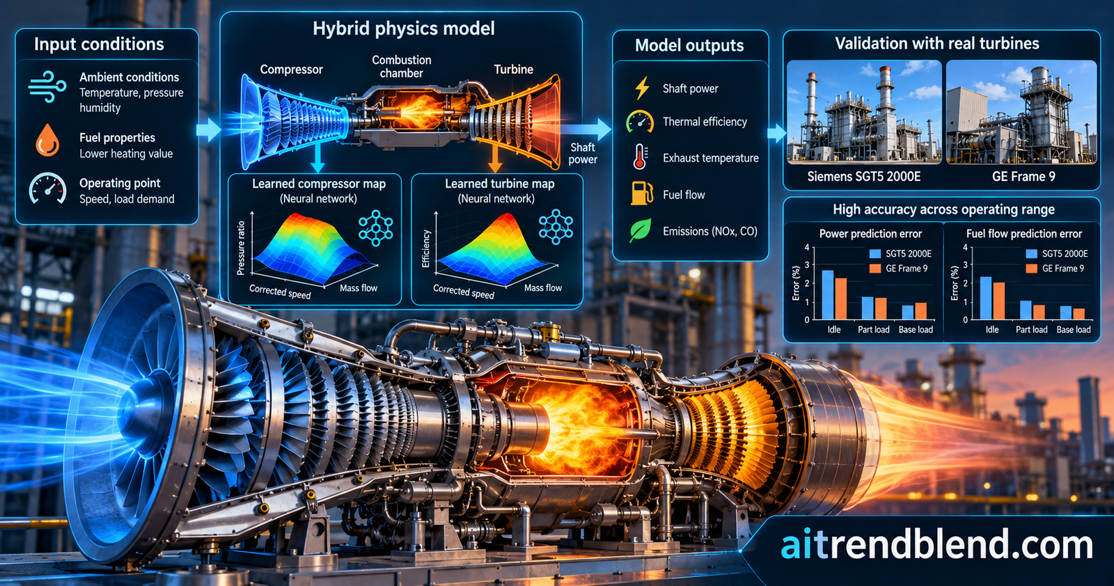
The most important temperature in a gas turbine is one nobody can measure. The gas entering the first turbine stage is hotter than a thermocouple would survive, and the air flowing through the compressor has no meter either. Engineers estimate both from heat balances, using the fuel flow, the fuel’s heating value and a handful of ordinary temperatures and pressures. If the fuel flowmeter is a little off, every estimate built on it is off too.
Hadi Zare Jafari and Amir Zanj at Flinders University in Adelaide built a modelling framework around that awkward fact. Their open access paper in Engineering Applications of Artificial Intelligence keeps the thermodynamics of a gas turbine as fixed physics and trains four small neural networks to supply only the compressor and turbine characteristic maps. It also adds a rule that checks two fuel flowmeters against each other. This article explains how the pieces fit, what the error figures mean, and where the evidence stops.
Key points
- Four one hidden layer networks, holding between 7 and 17 neurons each on the SGT5 2000E, replace the compressor and turbine flow and efficiency maps inside a physics model. A Newton Raphson solver finds compressor and turbine pressure ratios and fuel flow, taking about 0.18 seconds per steady state point on a standard workstation CPU with no GPU.
- On a random 20 percent test split the maps reach a mean relative error of 0.18 to 0.63 percent on the SGT5 2000E (2721 points) and 0.27 to 0.76 percent on the GE Frame 9 (1832 points).
- With whole operating regimes held out, the largest cell in the paper’s heat maps is 1.15 percent on the SGT5 2000E and 0.90 percent on the Frame 9, both under cold ambient exclusion. The integrated outputs in the benchmark figures reach about 1.5 percent, which the abstract does not mention.
- A fuel consistency rule drops data when base load turbine inlet temperature from gas and from liquid fuel differs by 4 °C or more. The paper does not report how many points it removed.
- Two of the four evaluated outputs, air flow and turbine inlet temperature, are themselves soft sensor estimates. The authors cannot share the data, and no code is released.
Why the maps are the whole game
A gas turbine simulation built by component matching treats the machine as a chain of parts. Air enters through the intake, the compressor raises its pressure, fuel burns in the combustor, the hot gas expands through the turbine, and the exhaust leaves through a duct. Each part obeys textbook thermodynamics. The unknowns are found by demanding that mass, pressure and power all balance where the parts meet. The paper calls this the dominant physics based strategy and builds on a simulation study of a twin shaft industrial turbine by Mohammadian and Saidi, whose model the authors simplify into a generic skeleton.
What the textbook equations cannot supply is the behaviour of the blades. For a given corrected speed and pressure ratio, how much air does the compressor pass, and how efficiently? The same two questions apply to the turbine. The answers live in characteristic maps. Maps usually come from rig tests, manufacturer data or CFD, and the paper points out that the accuracy of a component matching model is limited by how faithful they are. A real machine also differs from its datasheet, so an engineer who wants a model of this particular turbine needs maps fitted to its own field data.
That is the gap the authors target. They sort hybrid gas turbine models into three families, and the family they join is the third.
| Hybrid family | What the network does | Where generalization comes from | Examples the paper names |
|---|---|---|---|
| Surrogate | Imitates the outputs of a physics model, so it runs fast | The physics model that generated its training data | Liu and Karimi 2020, Jiang and colleagues 2025 |
| Residual learning | Learns the gap between the physics model and field data | The physics model underneath, left unchanged | Xu and colleagues, 2020 to 2023 |
| Performance adaptation | Tunes internal parameters of the physics model, most influentially the component maps | The physics skeleton, which the tuned maps plug into | Tsoutsanis 2014, Zhang 2024, Liu 2026, and this paper |
Families as described in the introduction of the paper. The table paraphrases the authors’ own sorting.
The novelty claim is carefully worded. The authors say they are, to the best of their knowledge, the first to replace the compressor and turbine maps of a heavy duty gas turbine with data driven surrogates while extending coverage beyond the compressor and keeping every input and output of the original maps. Their Table 1 supports this by listing seven earlier neural network adaptation studies from 2009 to 2026 and marking each as partial or absent on the turbine side, on consistency with the physics model, or on checking fuel data. Read the claim as a conjunction. Compressor only work, partial turbine work and unconstrained black box models all exist already. What is new is the combination, judged by the authors’ own definition of consistent. The last column of that table, a check on fuel heterogeneity, says no for every earlier study, which is unsurprising because the check is the authors’ own contribution.
The instinct to keep the physics fixed and let data fill only the unknown part runs through other work on this site. One example is a physics informed estimate of coronary flow reserve, and another is a wave simulator that generates paired ultrasound training data. In the turbine paper the unknown part is unusually small and well defined, four curves, which is what makes the idea attractive.
The skeleton and its four learned maps
The skeleton has five parts, namely the air intake, compressor, combustion chamber, turbine and exhaust channel. Ambient pressure, temperature and humidity, together with the load setpoint, are the boundary conditions. The authors ignore heat soakage, shaft dynamics and actuator dynamics, so the model describes steady states only. Turbine cooling is handled implicitly through a virtual turbine inlet temperature, which ISO 2314 defines as the equivalent mean temperature of an uncooled turbine. The inlet air is a mixture of five gases, oxygen, water vapour, carbon dioxide, nitrogen and argon, and all gases are treated as ideal.
The four learned maps enter through corrected variables. Corrected speed and corrected flow remove the effect of inlet temperature and pressure, so one map serves a hot afternoon and a cold morning. The compressor maps also take the position of the inlet guide vanes, because the vanes shift every speed line. The turbine maps take corrected speed and pressure ratio only.
Everything else is physics. The table below shows who owns what.
| Part | Physics, written by hand | Learned |
|---|---|---|
| Air intake | Pressure drop that grows with the square of corrected flow (Eqs. 1 to 3) | Nothing |
| Compressor | Outlet temperature and pressure from efficiency, and shaft power consumed (Eqs. 6 to 8) | Corrected flow and isentropic efficiency |
| Combustor | Energy balance with combustion efficiency and fuel heating value, and equal compressor outlet and turbine inlet pressure (Eqs. 9 and 10) | Nothing |
| Turbine | Exhaust pressure, exhaust enthalpy and power produced (Eqs. 13 to 16) | Corrected flow and isentropic efficiency |
| Exhaust channel | Pressure loss, computed like the intake | Nothing |
| Control logic | Exhaust temperature limiter and inlet guide vane behaviour (Eqs. 20 and 24 to 26) | Nothing |
Division of labour in the skeleton, from Section 2.1 and Section 2.3 of the paper.
Equations 4, 5, 11 and 12 number the networks as compressor flow, compressor efficiency, turbine flow and turbine efficiency. The text around Table 8 and the heat maps numbers them as compressor efficiency, compressor flow, turbine efficiency and turbine flow. The baseline cells of the heat maps match the second order. This article names maps by function wherever it can, and uses the second numbering only when it quotes those tables.
Three equations close the system, and the third changes with the operating mode. The first is mass conservation in the combustor, where air plus fuel must equal the gas flow the turbine map accepts. The second is pressure continuity through the machine. At part load the third equation is the power balance on the third line of the box, where turbine power minus compressor power, losses and generator demand must vanish. The demand on the next line is a requested percentage of the base load power, which the model computes first. At base load the third equation is the last line instead, and it says the turbine exhaust temperature equals a limit that the control system enforces.
The control logic is written by hand
The base load limiter is where the physics skeleton meets the vendor’s control system, and the paper gives the logic for each turbine. On the GE Frame 9 the exhaust temperature setpoint falls linearly with compressor discharge pressure. The maximum is 567 °C, the slope is 16.6 °C per bar, and the corner sits at 8 bar. On the SGT5 2000E the limit depends on compressor inlet temperature, with a fixed value of 536 °C, a 20 °C correction at base load and a 2 °C correction in combined cycle. The authors take these from vendor documents. That matters for anyone hoping to reuse the framework, because the learned part does not remove the need for the control documentation of each new machine.
Solving it with Newton Raphson
The paper’s Algorithm 1 is short. For each operating point the program fixes ambient conditions, load and fuel composition, then starts the unknown vector of compressor pressure ratio, turbine pressure ratio and fuel flow at their design point values. In every iteration it forms the compressor map inputs from the current guess, evaluates the two compressor networks, applies the compressor equations, runs the combustor balance, forms the turbine map inputs, evaluates the two turbine networks, applies the turbine equations and collects the three residuals. A Newton step then updates the unknowns, and the loop ends when every residual is below one millionth or after 100 iterations.
The networks sit inside the loop and not before it, which is the point of the design. The authors report the cost on an Intel Core i5 at 2.6 GHz with 16 GB of memory and no GPU. Training the four networks took on average 7.93 seconds for the SGT5 2000E and 4.87 seconds for the Frame 9, and solving a single steady state point took 0.182 and 0.194 seconds. Those are small numbers, and they describe a steady state calculation on a desktop. They do not describe a transient controller or an online estimator, and the paper does not claim they do.
One gap is worth knowing about. In the first iteration the guide vane position gets an initial value, and in later iterations it is set by the control logic, but the paper does not write the part load vane schedule as an equation. Our reference code supplies a made up schedule, and says so. A second, our own reading, concerns smoothness. The Jacobian is built through the networks, so a learned map has to be smooth between its training points. A curve that wiggles between samples could send the solver somewhere odd even when the fit looks excellent on the training data. The paper gives no convergence statistics. In our toy run every solve converged, which proves little about a real machine.
The design buys two things at once. The balance laws guarantee that mass, pressure and energy add up for any input the solver can reach, and the networks absorb the part that no datasheet captures, the behaviour of this machine’s blades. The price is a fixed skeleton that must match the real engine’s layout and control logic.
Soft sensors, and the fuel flowmeter problem
The framework starts from 19 raw sensor channels, listed in the paper’s Tables 2 and 5, with the permissible uncertainties that ISO 2314 sets. Ambient temperature is good to 0.2 °C, generator power to 0.2 percent, exhaust temperature to 3 °C, and liquid fuel flow to 0.5 percent. For gas fuel the standard gives a combined 0.5 percent covering temperature, pressure, volumetric flow and composition. The GE Frame 9 carries 24 exhaust thermocouples and six ambient temperature sensors, because redundancy is the authors’ answer to drifting instruments.
Three variables that the model needs cannot be measured in a running turbine, namely compressor air flow, turbine gas flow and turbine inlet temperature. The authors estimate them with the heat and mass balance methods of ISO 2314 and ASME PTC 22, which need no CFD. The methods do need laboratory analysis of the fuel, covering composition, lower heating value and density. That is why the fuel measurement has such influence over everything downstream.
“Accurate fuel flow measurement is essential, as erroneous readings directly affect calculations of TIT, air mass flows, and overall cycle efficiency.”Zare Jafari and Zanj, Section 2.2.4
A rule that uses the machine’s own physics
The authors’ answer to unreliable flowmeters has two parts. The first is calibration. The second is a consistency rule that exploits plants running on two fuels. Under base load the control system holds the thermal load on the turbine steady, so turbine inlet temperature should come out about the same whichever fuel is burning. The paper supports this with a simulation from the earlier Mohammadian and Saidi study.
| Fuel | Lower heating value (kJ/kg) | Power (kW) | Exhaust temperature (°C) | Turbine inlet temperature (°C) |
|---|---|---|---|---|
| Gas | 50,047 | 25,400 | 540.9 | 1115.2 |
| Liquid | 42,600 | 24,770 | 540.9 | 1115.0 |
Design point simulation at 15 °C, 1.01325 bar and 60 percent relative humidity, reproduced from Table 3 of the paper, which takes it from earlier simulation work and not from the authors’ own machines.
Switching to the lower energy fuel costs 630 kW of output in that simulation, about 2.5 percent by our subtraction, yet the inlet temperature moves by 0.2 °C. The validation rule turns that observation into a filter. If the turbine inlet temperature computed from gas fuel data and from liquid fuel data at base load differ by more than a threshold, at least one flowmeter is wrong, and the data are discarded.
It is an economical idea. The check costs no extra instrument, it uses an invariant the machine already provides, and it targets the sensor the authors rate as most error prone. It also deserves a closer look, because the paper leaves several practical questions open.
The first is the threshold. Four degrees is 0.36 percent of a 1115 °C inlet temperature by our arithmetic, and it is twenty times the 0.2 °C gap in the design simulation. The paper justifies it as lying within allowable measurement uncertainty in industrial codes and cites Xu and colleagues 2023. By its own reference list, that work is a paper on an adaptive onboard model for gas turbine engines, not a measurement standard. What a 4 °C gap means in flowmeter terms is not stated. In our toy plant, described in the code section, a 1 percent fuel flow error moves the soft sensor inlet temperature by 2.9 K, so a 4 K gate would catch errors of roughly 1.4 percent and pass those near the 0.5 percent uncertainty class. A real turbine has a different sensitivity, so that number does not transfer. The lesson is that a threshold should be tied to a flow error budget, and the paper does not do that.
The second is the pairing. The rule needs gas and liquid points at comparable conditions, and the paper does not say how comparable is decided, whether by ambient temperature, by date or by test campaign. The third is what gets thrown away. A disagreement cannot say which meter is wrong, so a faithful implementation might discard both sides. The paper says only that data failing the check are filtered out. The fourth is how many points that was. The dataset sizes in Table 6 are 2721 and 1832, but the number removed is not reported, so a reader cannot tell whether the rule touched 1 percent of the data or 30 percent. The fifth is reach. The rule checks base load only and applies only to turbines with two fuels. A plant that burns gas alone cannot use it, and a flowmeter that drifts only at part load escapes it.
Cross checking two instruments through a physical invariant is a sound and cheap idea, and it scales to any plant with redundant paths. It detects disagreement and nothing more. Whether it protects the learned maps depends on a threshold, a pairing rule and a count of removed points that the paper does not give.
Three levels of data fusion
The paper describes its fusion of heterogeneous data at three levels. At the data level it concatenates operational logs, dedicated tests and laboratory fuel analyses into one table. The tests are planned to fill gaps that normal operation leaves. A turbine spends long stretches at base load, so the authors add part load, peak load, guide vane sweeps from minimum opening to fully open, hot and cold days, both fuels, and for the Frame 9 both simple and combined cycle. The two datasets hold 2721 instances with 21 features for the SGT5 2000E and 1832 instances with 19 features for the Frame 9.
At the feature level the authors choose dimensionless variables that do not depend on fuel or cycle. From 19 raw channels they build nine features, the corrected flow, corrected speed, pressure ratio and efficiency of each component, plus guide vane position. The turbine efficiency comes from enthalpies at the turbine inlet, so it depends on the soft sensor estimate of inlet temperature.
The argument is that features of this kind let knowledge cross boundaries. Insight gained on liquid fuel should carry to gas fuel without retraining, and simple cycle data should inform combined cycle. At the validation level the Eq. 21 rule closes the loop. The claim is testable, and the paper tests it by leaving data out.
What the numbers say
Map accuracy on a random split
The four networks have one hidden layer each. The authors scanned 1 to 20 neurons per network and settled on 7 to 17 for the SGT5 2000E and 9 to 14 for the Frame 9. By our count the largest of these has 86 parameters, so the whole learned part of the model is a few hundred numbers. Training used Bayesian regularization with a Levenberg Marquardt style update plus early stopping, and the data were split 80 and 20 by a stratified shuffle method. The next table gives the paper’s whole dataset row from Table 8, with maps named by function.
| Learned map | SGT5 2000E, MRE (%) | GE Frame 9, MRE (%) | ||
|---|---|---|---|---|
| Train | Test | Train | Test | |
| Compressor efficiency | 0.33 | 0.33 | 0.49 | 0.51 |
| Compressor corrected flow | 0.34 | 0.36 | 0.43 | 0.47 |
| Turbine efficiency | 0.48 | 0.50 | 0.67 | 0.69 |
| Turbine corrected flow | 0.26 | 0.27 | 0.50 | 0.53 |
Entire dataset rows of Table 8. Across all 56 test cells in that table the range is 0.18 to 0.76 percent. By our scan of the table the largest test minus train difference is 0.11 percentage points, tighter than the 0.4 the text says is typical.
These are good numbers, and the train and test columns are almost identical. On its own, that pattern is only mildly informative, for reasons the critique below spells out. The authors also report that gas and liquid fuel rows differ by typically under 0.05 percentage points, which fits their claim that the features are fuel independent.
Leaving whole regimes out
The more telling test is the paper’s set of exclusion scenarios. In each one a slice of operating data is removed from training and the model is scored on that slice. Scenario 1 removes all liquid fuel data. Scenario 2 removes part load between 70 and 80 percent. Scenario 3 removes negative ambient temperatures. Scenario 4 removes 80 percent of the simple cycle data, and Scenario 5 removes a composite of pieces of the earlier exclusions. The next table reproduces the values the paper prints in its two heat maps, which it labels by network.
| Scenario | SGT5 2000E, MRE (%) | GE Frame 9, MRE (%) | ||||||
|---|---|---|---|---|---|---|---|---|
| ANN1 | ANN2 | ANN3 | ANN4 | ANN1 | ANN2 | ANN3 | ANN4 | |
| Baseline | 0.33 | 0.34 | 0.49 | 0.26 | 0.49 | 0.44 | 0.67 | 0.51 |
| 1, liquid fuel out | 0.34 | 0.48 | 0.49 | 0.60 | 0.53 | 0.55 | 0.71 | 0.63 |
| 2, load 70 to 80 percent out | 0.37 | 0.36 | 0.50 | 0.41 | 0.53 | 0.51 | 0.72 | 0.52 |
| 3, negative ambient out | 1.15 | 0.98 | 0.67 | 0.68 | 0.86 | 0.78 | 0.90 | 0.78 |
| 4, simple cycle mostly out | 0.33 | 0.43 | 0.51 | 0.39 | 0.50 | 0.50 | 0.73 | 0.54 |
| 5, composite out | 0.32 | 0.38 | 0.49 | 0.38 | 0.50 | 0.48 | 0.69 | 0.49 |
Values read from the heat maps in Figures 9 and 10 of the paper, which print them to two decimals and label the rows ANN1 to ANN4. The baseline cells equal the map level values of Table 8, in the order compressor efficiency, compressor flow, turbine efficiency and turbine flow. The two highlighted cells are the maxima the abstract quotes.
Three things stand out. Cold ambient exclusion is the hardest case, with the first SGT5 2000E cell rising from 0.33 to 1.15 percent, a factor of 3.5. Part load exclusion barely registers, which is plausible because the gap sits between operating points the networks have seen. And removing liquid fuel is not free. On the SGT5 2000E the fourth cell goes from 0.26 to 0.60 percent and the second from 0.34 to 0.48. If the features were perfectly fuel independent, those cells would not move. They move modestly, which tells us the independence is good and not exact.
There is a mechanical reason that cold weather hurts most. Corrected speed is shaft speed divided by the square root of inlet temperature, so a cold day raises it. Removing the cold days therefore pushes the compressor map inputs outside the range seen in training, while removing a load band leaves them inside. The paper does not make this point, and our toy run later in the article shows it directly.
Against other models
The paper then compares the integrated model against three alternatives on the final outputs, which are compressor outlet temperature T3, air mass flow, turbine exhaust temperature and turbine inlet temperature. They are an XGBoost model with 300 boosting rounds, trees of depth up to 20 and a learning rate of 0.05, a Deep MLP, and a hybrid called MVIAC that mainly adapts the compressor maps and only partly the turbine maps. The benchmark section describes a 70, 15 and 15 percent split for training, validation and testing, which differs from the 80 and 20 split of the main model.
| Model | What it is | Worst errors the paper reports |
|---|---|---|
| Learned maps in physics skeleton | This paper | About 0.3 to 1.0 percent on the Frame 9 and 0.3 to 1.54 percent on the SGT5 2000E across six scenarios and four outputs |
| MVIAC | Hybrid, compressor maps adapted, turbine maps partly | About 1.8 percent on exhaust temperature and 1.6 percent on air flow (SGT5 2000E), 1.4 percent on exhaust temperature (Frame 9) |
| XGBoost | Purely data driven | Air flow 6.09 percent (Frame 9) and 9.02 percent (SGT5 2000E) when liquid fuel is excluded, about 3.4 and 4.9 percent when cold days are excluded |
| Deep MLP | Purely data driven | Below 1.6 percent on the full data, up to about 5.01 and 9.67 percent when liquid fuel is excluded, about 3.2 and 3.8 percent for cold days |
Figures quoted from Section 3.2.2 of the paper. The paper does not list the inputs of the data driven baselines.
The picture is striking for the data driven models. When liquid fuel disappears from training, air flow error balloons to 5 to 10 percent, roughly ten times the hybrid’s. That is the strongest evidence in the paper that embedding physics buys extrapolation.
The bar charts say something subtler, which is worth reading closely. The text says the proposed framework consistently achieves the lowest errors among all evaluated methods. The bars do not always show that. By our reading of Figures 11 to 13, accurate to roughly a tenth of a point, the XGBoost bars sit below the hybrid on the Frame 9 baseline for T3 (about 0.37 against 0.46), exhaust temperature (0.44 against 0.59) and inlet temperature (0.29 against 0.43). Under Scenario 2 on the Frame 9 the Deep MLP is lower for exhaust temperature (about 0.46 against 0.63) and inlet temperature (0.30 against 0.44). On the SGT5 2000E under cold exclusion the hybrid’s T3 error, about 1.55, is above MVIAC at about 1.45 and the Deep MLP at about 1.25. Black box models interpolate well. What the physics skeleton buys is robustness where the data stop, and it does not buy a lower error everywhere.
Judge a hybrid model by its worst case outside the training range and not by its best case inside it. On that test the paper’s physics skeleton clearly wins against black boxes, with air flow errors under 1.1 percent where the others reach 5 to 10 percent. Inside the training range a plain model can be just as accurate.
Where the claims stretch
Two of the four references are estimates
Equation 27 defines the error against a measured or reference value. Compressor air flow and turbine inlet temperature cannot be measured, so their reference is the ISO 2314 soft sensor, the same machinery that built the training features. The reported errors for those two outputs therefore measure agreement with an estimator and not with the machine. Any systematic bias in that estimator, such as a fuel flow offset the Eq. 21 rule missed, would be learned faithfully and score well. Table 5 allows 0.5 percent uncertainty in fuel flow, which is on the same scale as the 0.3 to 0.7 percent map errors. In our toy plant the soft sensor’s own error against the exact truth is 0.20 percent for inlet temperature and 0.79 percent for air flow with instrument noise set near the levels of the paper’s Table 5, which is as large as the map errors the paper reports.
The random split rewards near neighbours
The headline test results come from a random 80 and 20 split. The paper itself says operational data are often similar or closely related, with long runs at base load. A random split puts neighbours of each test point into the training set, so the test measures interpolation among points that nearly repeat. The paper does not describe splitting by date or by test campaign, which would be tougher. It also describes early stopping on a validation loss without saying where the validation points come from, and it does not say whether the neuron sweep in Figure 6 scored test or validation error. If the sweep used test error, the selected sizes are mildly optimistic. These are questions of reporting, and the data are not available to settle them.
Which number is the headline
The abstract quotes up to 1.15 percent for the SGT5 2000E and 0.9 percent for the Frame 9. Those match the largest cells of the two heat maps, and the conclusion repeats the 1.15 figure. The integrated outputs in the benchmark figures go higher. The proposed model’s T3 error on the SGT5 2000E under cold exclusion is about 1.54 percent in Figure 11, and Section 3.2.2 itself gives a range of 0.3 to 1.54 percent. There is also a labelling puzzle. Section 3.2.1 says the evaluated variables are compressor air flow, compressor outlet temperature and the two turbine temperatures, yet the heat maps are labelled by network. For the Frame 9 under Scenario 3 the four cells (0.86, 0.78, 0.90 and 0.78) equal, to the precision we can read from the bars, the T3, air flow, exhaust temperature and inlet temperature bars of Figure 11, while the baseline cells equal the map level values of Table 8. We could not tell from the text what each cell holds. Either way, 1.15 percent is not the largest error the paper’s own figures show.
Interpretable means the skeleton
The title promises a physics interpretable model. What is interpretable is the structure. A reader can see which equation computes compressor power and where the exhaust limiter acts. The learned maps themselves are one hidden layer networks, and none of the paper’s thirteen figures plots a learned map against what an engineer expects, such as speed lines bending toward surge. A claim that the maps are physically sensible, as opposed to numerically accurate, is untested in the text. That is easy to fix and would strengthen the paper.
Scope
Both turbines are heavy duty machines. The paper does not state the site, the period over which data were collected or whether any of it spans a major overhaul, and it does not discuss gradual degradation of the engine such as fouling. A map fitted this year may drift next year, and the framework as published has no mechanism for tracking that. The authors list uncertainty quantification and deployment across more turbines as future work.
A steady state model with 0.3 to 1.5 percent error is a sound base for performance analysis, benchmarking and anomaly screening. It is not shown to be fit for protection or trip logic, where dynamics, sensor faults and certification matter, and the paper itself targets performance analysis and condition monitoring. Anyone adapting the approach to a real plant should keep it advisory until it has been validated against that plant’s own acceptance tests.
Limitations the paper states, and the ones it leaves open
The authors state one limitation directly. The framework targets steady state performance across part load and base load, and it deliberately leaves out shaft dynamics, heat soakage and actuator effects. They suggest adding rotor inertia and control dynamics later for hybrid steady and transient simulation, and they name uncertainty quantification and broader fleet deployment as next steps.
Several limits are visible in the numbers. The evidence rests on two turbines, 2721 and 1832 operating points, and a single set of exclusion scenarios. Cold ambient exclusion lifts the largest heat map cell to 1.15 and 0.90 percent from baseline cells of 0.26 to 0.67. Liquid fuel exclusion raises one SGT5 2000E cell from 0.26 to 0.60 percent. The benchmark bars show the data driven models winning some baseline cells, and the soft sensor reference for two of the four outputs has its own uncertainty that the paper does not propagate.
“The authors do not have permission to share data.”Zare Jafari and Zanj, Data availability statement
The last limit is access. The data availability statement says the data cannot be shared, and the paper points to no code. Nobody outside the authors can rerun the exclusion scenarios, change the threshold of the fuel rule or test a different split. For a paper whose main claim is generalization, an independent check is the natural next step, and the code section below builds a small version of one on invented data.
A PyTorch version on an invented plant
The paper shares neither data nor code, so nothing here can reproduce its numbers. What can be rebuilt is the structure, and structure is where this paper is most instructive. The file below is our own independent reconstruction from the paper’s text and equations. It is not the authors’ code. It builds a toy gas turbine of our own, solves it with the same three unknowns and the same Newton Raphson loop, replaces its four characteristic maps with one hidden layer networks, and runs a miniature version of the paper’s experiments on invented operating data.
Several choices are ours, and the code marks each as a design choice. The gas is calorically perfect and not a five species mixture. The part load guide vane schedule is invented because the paper gives none. The pairing rule for the fuel check is ours, and so is dropping both sides of a failing pair. Training uses Adam with weight decay and an early stopping split in place of the paper’s Bayesian regularization. The data come from campaigns of 110 points in gas and liquid pairs, with one liquid flowmeter given a 2 percent bias on purpose.
"""
gasturbine_hybrid_reference.py
Independent, educational reconstruction of the hybrid gas turbine idea in
Zare Jafari and Zanj, Engineering Applications of Artificial Intelligence 184 (2026) 116284.
This is NOT the authors' code. The paper shares neither code nor data, so everything
numeric below runs on a TOY plant that we invented. Nothing here reproduces their numbers.

Faithful to the paper's text (checked against its equations):
  * a steady state component matching skeleton: intake, compressor, combustor, turbine, exhaust
  * only the four characteristic maps are learned (ANN1 to ANN4, one hidden layer each)
  * unknowns x = [PRc, PRt, mf], solved by Newton Raphson from design point values, tol 1e-6, 100 iterations
  * residuals: mass balance (Eq 17), pressure continuity (Eq 18), part load power balance (Eq 19)
    or a turbine exhaust temperature limiter at base load (Eq 20, GE Frame 9 style Eq 24 constants)
  * soft sensors from an energy balance, corrected speed and efficiency features (Eqs 22, 23)
  * physics consistent fuel cross check of base load TIT, gas against liquid, 4 C threshold (Eq 21)
  * extrapolation tests that exclude liquid fuel, 70 to 80 percent load, and cold ambient
DESIGN CHOICES marked below are ours, because the paper does not specify them.
"""
import time
import torch
import torch.nn as nn

torch.set_default_dtype(torch.float64)

# ---------------------------------------------------------------- constants (toy)
CP_A, G_A = 1005.0, 1.4          # air, calorically perfect (DESIGN CHOICE: the paper uses a five gas mixture)
CP_G, G_G = 1160.0, 1.33         # combustion gas
ETA_CC = 0.99
LHV = {"gas": 50_047e3, "liquid": 42_600e3}   # J/kg, the two fuels in the paper's Table 3
W_LOSS = 1.5e6                    # W, mechanical and generator loss (DESIGN CHOICE: constant)
PF = 1.0                          # Eq 19 prints Wgen/PF. We keep the printed form with PF = 1
T_REL, TIT_REL = 288.15, 1350.0   # reference temperatures for relative corrected speeds
MC_D = 6.9                        # design corrected compressor flow (scaled units)
X0 = torch.tensor([12.0, 10.5, 6.0])  # design point start for [PRc, PRt, mf]


def t7_limit(cpd_bar):
    """Eq 24 with the paper's GE Frame 9 constants: 567 C max, 16.6 C per bar, corner at 8 bar. Returns kelvin."""
    return 273.15 + 567.0 - 16.6 * torch.clamp(cpd_bar - 8.0, min=0.0)


def igv_schedule(pl):
    """DESIGN CHOICE: the paper says control logic sets the IGV but gives no schedule. Ours closes it below 80 percent load."""
    return torch.clamp(0.62 + 0.38 * (pl - 0.4) / 0.4, 0.62, 1.0)


# ---------------------------------------------------------------- characteristic maps
class TrueMaps:
    """The hidden plant. Analytic toy maps that play the role of the real machine."""
    def comp(self, nc, pr, igv):
        pr_ref = 1.0 + 11.0 * nc ** 2.2
        z = pr / pr_ref - 1.0
        mc = MC_D * (0.5 + 0.5 * igv) * (0.25 + 0.75 * nc) * (1.0 - 0.5 * z)
        eta = 0.88 - 1.2 * z ** 2 - 0.2 * (nc - 1.0) ** 2 - 0.05 * (1.0 - igv)
        return mc, eta

    def turb(self, nt, pr):
        mtc = 1.29 * torch.tanh(0.62 * torch.sqrt(pr - 1.0)) * (1.0 + 0.05 * (nt - 1.0))
        eta = 0.90 - 0.45 * (nt - 1.0) ** 2 - 0.0015 * (pr - 10.5) ** 2
        return mtc, eta


class MapNet(nn.Module):
    """One hidden layer MLP with built in input and output scaling, as in the paper's ANN1 to ANN4."""
    def __init__(self, n_in, n_hidden):
        super().__init__()
        self.l1, self.l2 = nn.Linear(n_in, n_hidden), nn.Linear(n_hidden, 1)
        self.register_buffer("xm", torch.zeros(n_in)); self.register_buffer("xs", torch.ones(n_in))
        self.register_buffer("ym", torch.zeros(1)); self.register_buffer("ys", torch.ones(1))

    def fit_scale(self, X, y):
        self.xm.copy_(X.mean(0)); self.xs.copy_(X.std(0) + 1e-9)
        self.ym.copy_(y.mean()); self.ys.copy_(y.std() + 1e-9)

    def forward(self, X):
        z = (X - self.xm) / self.xs
        return self.l2(torch.tanh(self.l1(z))).squeeze(-1) * self.ys + self.ym


class HybridMaps:
    """Eqs 4, 5, 11, 12: the four learned maps behind the same interface as TrueMaps."""
    def __init__(self, nets):
        self.n1, self.n2, self.n3, self.n4 = nets

    def comp(self, nc, pr, igv):
        X = torch.stack([nc, pr, igv], -1)
        return self.n1(X), self.n2(X)

    def turb(self, nt, pr):
        X = torch.stack([nt, pr], -1)
        return self.n3(X), self.n4(X)


# ---------------------------------------------------------------- the physics skeleton
def states(x, c, maps):
    """Everything downstream of x = [PRc, PRt, mf] for a batch of operating points c."""
    prc, prt, mf = x[:, 0], x[:, 1], x[:, 2]
    T2, P0, igv = c["T0"], c["P0"], c["igv"]
    nc = torch.sqrt(T_REL / T2)                                   # corrected speed, relative
    mc, eta_c = maps.comp(nc, prc, igv)                           # ANN1, ANN2 (Eqs 4, 5)
    dp_in = 0.01 * (mc / MC_D) ** 2                               # Eqs 1 to 3 simplified (DESIGN CHOICE: uses mc, no lag)
    P2 = P0 * (1.0 - dp_in)
    ma = mc * 1e3 * P2 / torch.sqrt(T2)                           # kg/s, P in bar
    T3 = T2 * (1.0 + (prc ** ((G_A - 1) / G_A) - 1.0) / eta_c)    # Eqs 6, 7
    P3 = P2 * prc                                                 # Eq 8
    WC = ma * CP_A * (T3 - T2)
    TIT = (ma * CP_A * T3 + mf * ETA_CC * c["lhv"]) / ((ma + mf) * CP_G)   # Eq 9, fuel sensible heat ignored
    P6 = P3                                                       # Eq 10
    nt = torch.sqrt(TIT_REL / TIT)
    mtc, eta_t = maps.turb(nt, prt)                               # ANN3, ANN4 (Eqs 11, 12)
    mg = mtc * 1e3 * P6 / torch.sqrt(TIT)
    T7 = TIT * (1.0 + eta_t * (prt ** ((1 - G_G) / G_G) - 1.0))   # Eq 14
    WT = mg * CP_G * (TIT - T7)                                   # Eq 15
    P7 = P0 * (1.0 + 0.012 * (mg / 410.0) ** 2)                   # DESIGN CHOICE: exhaust duct drop, Eq 18 uses it
    return dict(ma=ma, mg=mg, T3=T3, P2=P2, P3=P3, P7=P7, TIT=TIT, T7=T7, WC=WC, WT=WT, mf=mf, nc=nc, nt=nt)


def residual(x, c, maps):
    s = states(x, c, maps)
    r1 = (s["ma"] + s["mf"] - s["mg"]) / 410.0                    # Eq 17
    r2 = (s["P2"] * x[:, 0] - x[:, 1] * s["P7"]) / c["P0"]        # Eq 18
    part = (s["WT"] - c["wgen"] / PF - W_LOSS - s["WC"]) / 1e8    # Eq 19
    base = (s["T7"] - t7_limit(s["P3"])) / 100.0                  # Eqs 20, 24
    r3 = torch.where(c["base"], base, part)
    return torch.stack([r1, r2, r3], -1), s


def newton(c, maps, tol=1e-6, max_iter=100):
    """Algorithm 1: Newton Raphson from design values with a simple backtracking safeguard.
    The Jacobian comes from autograd through the ANN maps, so the maps sit inside every iteration."""
    B = c["T0"].shape[0]
    x = X0.repeat(B, 1).clone()
    for it in range(max_iter):
        x = x.detach().requires_grad_(True)
        F, _ = residual(x, c, maps)
        rows = [torch.autograd.grad(F[:, k].sum(), x, retain_graph=True)[0] for k in range(3)]
        J = torch.stack(rows, 1)
        nF = F.detach().abs().amax(1)
        if (nF < tol).all():
            break
        try:
            dx = -torch.linalg.solve(J, F.detach().unsqueeze(-1)).squeeze(-1)
        except RuntimeError:
            break
        best, best_n = x.detach(), nF
        for a in (1.0, 0.5, 0.25, 0.125, 0.0625, 0.03):
            xn = (x.detach() + a * dx)
            with torch.no_grad():
                Fn, _ = residual(xn, c, maps)
            nn_ = Fn.abs().amax(1)
            better = (nn_ < best_n) & torch.isfinite(nn_)
            best = torch.where(better.unsqueeze(-1), xn, best); best_n = torch.where(better, nn_, best_n)
        x = best
    with torch.no_grad():
        F, s = residual(x.detach(), c, maps)
    ok = F.abs().amax(1) < 1e-5
    return x.detach(), s, ok


def solve_plant(T0, P0, pl, fuel, maps):
    """Part load first needs the base load power, exactly as the paper describes."""
    n = T0.shape[0]
    lhv = torch.tensor([LHV[f] for f in fuel])
    cb = dict(T0=T0, P0=P0, igv=torch.ones(n), lhv=lhv, base=torch.ones(n, dtype=torch.bool), wgen=torch.zeros(n))
    xb, sb, okb = newton(cb, maps)
    wbl = sb["WT"] - sb["WC"] - W_LOSS
    isbase = pl >= 0.999
    c = dict(T0=T0, P0=P0, igv=igv_schedule(pl), lhv=lhv, base=isbase, wgen=pl * wbl)
    c["igv"] = torch.where(isbase, torch.ones(n), c["igv"])
    x, s, ok = newton(c, maps)
    s["wgen"] = s["WT"] - s["WC"] - W_LOSS
    return x, s, ok & okb, c


# ---------------------------------------------------------------- synthetic "plant data" (the paper's data are private)
def make_data(seed=0, n_pairs=8, per_campaign=110, flow_bias=0.02, biased_pair=3):
    """Campaigns come in gas and liquid pairs at the same ambient centre. One liquid campaign has a flowmeter bias."""
    g = torch.Generator().manual_seed(seed)
    centres = torch.linspace(-3.0, 38.0, n_pairs)
    rows = []
    for k in range(n_pairs):
        for fuel in ("gas", "liquid"):
            n = per_campaign
            T0 = 273.15 + centres[k] + (torch.rand(n, generator=g) - 0.5) * 5.0
            P0 = 1.013 + (torch.rand(n, generator=g) - 0.5) * 0.04
            base = torch.rand(n, generator=g) < 0.4
            pl = torch.where(base, torch.ones(n), 0.4 + 0.55 * torch.rand(n, generator=g))
            bias = flow_bias if (k == biased_pair and fuel == "liquid") else 0.0
            rows.append((T0, P0, pl, fuel, k, bias))
    T0 = torch.cat([r[0] for r in rows]); P0 = torch.cat([r[1] for r in rows]); pl = torch.cat([r[2] for r in rows])
    fuel = sum([[r[3]] * r[0].shape[0] for r in rows], [])
    camp = torch.cat([torch.full((r[0].shape[0],), 2 * r[4] + (r[3] == "liquid")) for r in rows])
    bias = torch.cat([torch.full((r[0].shape[0],), r[5]) for r in rows])
    x, s, ok, c = solve_plant(T0, P0, pl, fuel, TrueMaps())
    assert ok.all(), f"plant failed to converge for {int((~ok).sum())} points"
    nz = lambda scale, shape: torch.randn(shape, generator=g) * scale
    n = T0.shape[0]
    sens = dict(                                                   # what the instruments report (noise levels echo the paper's Table 5)
        T2=T0 + nz(0.2, n), P2=s["P2"] * (1 + nz(0.001, n)), T3=s["T3"] + nz(0.4, n), P3=s["P3"] * (1 + nz(0.001, n)),
        T7=s["T7"] + nz(1.5, n), P7=s["P7"] * (1 + nz(0.0005, n)), wgen=s["wgen"] * (1 + nz(0.002, n)),
        mf=s["mf"] * (1 + bias) * (1 + nz(0.005, n)), igv=c["igv"],
    )
    truth = dict(T3=s["T3"], ma=s["ma"], TET=s["T7"], TIT=s["TIT"])
    return dict(T0=T0, P0=P0, pl=pl, fuel=fuel, camp=camp, base=c["base"], sens=sens, truth=truth,
                lhv=c["lhv"], bias=bias)


def soft_sensors(d):
    """ISO 2314 flavoured heat balance, our toy version: air flow and TIT are not measured, they are computed
    from fuel flow, fuel LHV, power and temperatures. Their error therefore inherits the flowmeter error."""
    s, lhv = d["sens"], d["lhv"]
    wnet = s["wgen"] / PF + W_LOSS
    ma = (s["mf"] * ETA_CC * lhv - wnet - s["mf"] * CP_G * s["T7"]) / (CP_G * s["T7"] - CP_A * s["T2"])
    TIT = (ma * CP_A * s["T3"] + s["mf"] * ETA_CC * lhv) / ((ma + s["mf"]) * CP_G)
    return ma, TIT


def features(d):
    """Table 4 style features: dimensionless, independent of fuel and of operating mode. Eqs 22 and 23 give efficiencies."""
    s = d["sens"]; ma, TIT = soft_sensors(d)
    prc = s["P3"] / s["P2"]; prt = s["P3"] / s["P7"]
    nc = torch.sqrt(T_REL / s["T2"]); nt = torch.sqrt(TIT_REL / TIT)
    mc = ma * torch.sqrt(s["T2"]) / (1e3 * s["P2"])
    eta_c = s["T2"] * (prc ** ((G_A - 1) / G_A) - 1.0) / (s["T3"] - s["T2"])                   # Eq 22
    mtc = (ma + s["mf"]) * torch.sqrt(TIT) / (1e3 * s["P3"])
    eta_t = (TIT - s["T7"]) / (TIT * (1.0 - prt ** ((1 - G_G) / G_G)))                          # Eq 23
    return dict(nc=nc, prc=prc, igv=s["igv"], mc=mc, eta_c=eta_c, nt=nt, prt=prt, mtc=mtc, eta_t=eta_t, TIT=TIT, ma=ma)


# ---------------------------------------------------------------- Eq 21, physics consistent fuel cross check
def eq21_filter(d, F, threshold=4.0):
    """For each gas and liquid pair at comparable ambient, base load TIT must agree within `threshold` kelvin.
    DESIGN CHOICE: the paper does not say how pairs are formed or which side is dropped. We pair campaigns by
    ambient centre and, because the rule cannot say which flowmeter is wrong, drop both sides of a failing pair."""
    keep = torch.ones(d["T0"].shape[0], dtype=torch.bool); report = []
    for k in range(int(d["camp"].max().item()) // 2 + 1):
        mg = (d["camp"] == 2 * k) & d["base"]; ml = (d["camp"] == 2 * k + 1) & d["base"]
        dT = abs(F["TIT"][mg].mean() - F["TIT"][ml].mean()).item()
        failed = dT >= threshold
        report.append((k, dT, failed))
        if failed:
            keep &= ~((d["camp"] == 2 * k) | (d["camp"] == 2 * k + 1))
    return keep, report


# ---------------------------------------------------------------- training the four maps
def train_net(net, X, y, seed, epochs=900, lr=1e-2, wd=1e-6, patience=120):
    g = torch.Generator().manual_seed(seed)
    n = X.shape[0]; perm = torch.randperm(n, generator=g)
    nv = max(int(0.15 * n), 10); vi, ti = perm[:nv], perm[nv:]
    net.fit_scale(X[ti], y[ti])
    opt = torch.optim.Adam(net.parameters(), lr=lr, weight_decay=wd)   # DESIGN CHOICE: the paper uses Bayesian regularisation
    best, best_state, bad = 1e9, None, 0
    for ep in range(epochs):
        opt.zero_grad(); loss = ((net(X[ti]) - y[ti]) ** 2).mean(); loss.backward(); opt.step()
        with torch.no_grad():
            v = ((net(X[vi]) - y[vi]) ** 2).mean().item()
        if v < best - 1e-12:
            best, bad = v, 0; best_state = {k: t.clone() for k, t in net.state_dict().items()}
        else:
            bad += 1
            if bad > patience:
                break
    net.load_state_dict(best_state)
    return net


def train_maps(F, idx, seed=0, hidden=(12, 8, 12, 10)):
    Xc = torch.stack([F["nc"][idx], F["prc"][idx], F["igv"][idx]], -1)
    Xt = torch.stack([F["nt"][idx], F["prt"][idx]], -1)
    nets = [train_net(MapNet(3, hidden[0]), Xc, F["mc"][idx], seed),
            train_net(MapNet(3, hidden[1]), Xc, F["eta_c"][idx], seed + 1),
            train_net(MapNet(2, hidden[2]), Xt, F["mtc"][idx], seed + 2),
            train_net(MapNet(2, hidden[3]), Xt, F["eta_t"][idx], seed + 3)]
    return HybridMaps(nets)


def map_mre(maps, F, idx):
    """Per map relative error on held out points, the paper's Eq 27."""
    Xc = torch.stack([F["nc"][idx], F["prc"][idx], F["igv"][idx]], -1)
    Xt = torch.stack([F["nt"][idx], F["prt"][idx]], -1)
    with torch.no_grad():
        p = [maps.n1(Xc), maps.n2(Xc), maps.n3(Xt), maps.n4(Xt)]
    tg = [F["mc"][idx], F["eta_c"][idx], F["mtc"][idx], F["eta_t"][idx]]
    return [100 * ((a - b).abs() / b.abs()).mean().item() for a, b in zip(p, tg)]


# ---------------------------------------------------------------- baseline: a plain data driven model
class Direct(nn.Module):
    """Conditions straight to outputs, two hidden layers. A stand in for the paper's Deep MLP baseline."""
    def __init__(self):
        super().__init__()
        self.f = nn.Sequential(nn.Linear(4, 32), nn.Tanh(), nn.Linear(32, 32), nn.Tanh(), nn.Linear(32, 4))
        self.register_buffer("xm", torch.zeros(4)); self.register_buffer("xs", torch.ones(4))
        self.register_buffer("ym", torch.zeros(4)); self.register_buffer("ys", torch.ones(4))

    def forward(self, X):
        return self.f((X - self.xm) / self.xs) * self.ys + self.ym


def train_direct(d, F, idx, seed=0, epochs=1200):
    torch.manual_seed(seed)
    X = torch.stack([d["T0"], d["P0"], d["pl"], (torch.tensor([f == "liquid" for f in d["fuel"]])).double()], -1)
    Y = torch.stack([d["sens"]["T3"], F["ma"], d["sens"]["T7"], F["TIT"]], -1)
    net = Direct(); net.xm.copy_(X[idx].mean(0)); net.xs.copy_(X[idx].std(0) + 1e-6)
    net.ym.copy_(Y[idx].mean(0)); net.ys.copy_(Y[idx].std(0))
    n = idx.shape[0]; perm = idx[torch.randperm(n)]; nv = int(0.15 * n); vi, ti = perm[:nv], perm[nv:]
    opt = torch.optim.Adam(net.parameters(), lr=5e-3, weight_decay=1e-6)
    best, st, bad = 1e9, None, 0
    for ep in range(epochs):
        opt.zero_grad(); l = (((net(X[ti]) - Y[ti]) / net.ys) ** 2).mean(); l.backward(); opt.step()
        with torch.no_grad():
            v = (((net(X[vi]) - Y[vi]) / net.ys) ** 2).mean().item()
        if v < best - 1e-12:
            best, bad, st = v, 0, {k: t.clone() for k, t in net.state_dict().items()}
        else:
            bad += 1
            if bad > 150:
                break
    net.load_state_dict(st)
    return net, X


# ---------------------------------------------------------------- evaluation
def integrated_mre(maps, d, idx):
    """Run the whole skeleton with learned maps on held out conditions, compare with the noise free toy plant."""
    fuel = [d["fuel"][i] for i in idx.tolist()]
    _, s, ok, _ = solve_plant(d["T0"][idx], d["P0"][idx], d["pl"][idx], fuel, maps)
    tr = d["truth"]; out = {}
    for name, key, tk in (("T3", "T3", "T3"), ("Mf", "ma", "ma"), ("TET", "T7", "TET"), ("TIT", "TIT", "TIT")):
        ref = tr[tk][idx][ok]; est = s[key][ok]
        out[name] = 100 * ((est - ref).abs() / ref.abs()).mean().item() if ok.any() else float("nan")
    return out, ok.float().mean().item()


def direct_mre(net, X, d, idx):
    with torch.no_grad():
        p = net(X[idx])
    tr = d["truth"]
    refs = [tr["T3"][idx], tr["ma"][idx], tr["TET"][idx], tr["TIT"][idx]]
    return {k: 100 * ((p[:, j] - r).abs() / r.abs()).mean().item() for j, (k, r) in enumerate(zip(("T3", "Mf", "TET", "TIT"), refs))}


def outside_range(F, tr_idx, te_idx):
    """Share of held out compressor map inputs that fall outside the box of training inputs."""
    cols = ("nc", "prc", "igv")
    lo = torch.stack([F[c][tr_idx].min() for c in cols]); hi = torch.stack([F[c][tr_idx].max() for c in cols])
    X = torch.stack([F[c][te_idx] for c in cols], -1)
    return ((X < lo) | (X > hi)).any(-1).float().mean().item()


def fmt(dct):
    return "  ".join(f"{k} {v:5.2f}" for k, v in dct.items())


def main():
    t0 = time.time(); torch.manual_seed(0)
    # 1. the plant, its data, soft sensors and features
    d = make_data(seed=0); F = features(d); N = d["T0"].shape[0]
    print(f"toy plant data: {N} operating points, {int(d['base'].sum())} at base load, 8 gas and liquid campaign pairs")
    # sensitivity of the soft sensor reference to the flowmeter, in kelvin
    d2 = {**d, "sens": {**d["sens"], "mf": d["sens"]["mf"] * 1.01}}
    _, TIT1 = soft_sensors(d); _, TIT2 = soft_sensors(d2)
    print(f"soft sensor sensitivity: +1 percent fuel flow moves TIT by {(TIT2 - TIT1).mean().item():.1f} K "
          f"({100 * ((TIT2 - TIT1) / TIT1).mean().item():.2f} percent) and air flow by "
          f"{100 * ((soft_sensors(d2)[0] - soft_sensors(d)[0]) / soft_sensors(d)[0]).mean().item():.2f} percent")
    ref_err = 100 * ((F["TIT"] - d["truth"]["TIT"]).abs() / d["truth"]["TIT"]).mean().item()
    ref_ma = 100 * ((F["ma"] - d["truth"]["ma"]).abs() / d["truth"]["ma"]).mean().item()
    print(f"soft sensor reference vs exact toy truth, mean relative error: TIT {ref_err:.2f} percent, air flow {ref_ma:.2f} percent")

    # 2. Eq 21
    keep, rep = eq21_filter(d, F)
    print("Eq 21, base load TIT gas minus liquid per pair (K): " + ", ".join(f"{dT:.1f}{'*' if f else ''}" for _, dT, f in rep))
    print(f"    * fails the 4 K rule, so both campaigns of that pair are dropped, keeping {int(keep.sum())} of {N} points")

    # 3. baseline: random 80 / 20 split, with and without the filter
    g = torch.Generator().manual_seed(1); perm = torch.randperm(N, generator=g)
    test = perm[: N // 5]
    clean = (d["bias"] == 0)
    results = {}
    for name, usable in (("filtered by Eq 21", keep), ("unfiltered", torch.ones(N, dtype=torch.bool))):
        tr_idx = torch.tensor([i for i in perm[N // 5:].tolist() if usable[i]])
        te_idx = torch.tensor([i for i in test.tolist() if clean[i]])
        maps = train_maps(F, tr_idx, seed=0)
        m = map_mre(maps, F, te_idx); im, conv = integrated_mre(maps, d, te_idx)
        results[name] = (m, im, conv)
        print(f"baseline split, {name}: train n={len(tr_idx)}, map MRE ANN1..4 " + " ".join(f"{v:.2f}" for v in m))
        print(f"    integrated MRE (%) {fmt(im)}, solver converged {100 * conv:.0f}%")
    maps_base = train_maps(F, torch.tensor([i for i in perm[N // 5:].tolist() if keep[i]]), seed=0)

    # 4. exclusion scenarios, in the spirit of the paper's Scenarios 1 to 3 (toy has no cycle mode, so no 4 and 5)
    Tc = d["T0"] - 273.15
    liquid = torch.tensor([f == "liquid" for f in d["fuel"]])
    scen = {"S1 liquid fuel excluded": liquid,
            "S2 load 70 to 80 percent excluded": (d["pl"] >= 0.7) & (d["pl"] < 0.8),
            "S3 ambient below 5 C excluded": Tc < 5.0}
    print("\nexclusion scenarios, MRE (%) on the held out points against the noise free toy plant")
    for name, mask in scen.items():
        tr_idx = torch.where(keep & ~mask)[0]; te_idx = torch.where(mask & (d["bias"] == 0))[0]
        maps = train_maps(F, tr_idx, seed=0)
        im, conv = integrated_mre(maps, d, te_idx)
        net, X = train_direct(d, F, tr_idx, seed=0); dm = direct_mre(net, X, d, te_idx)
        print(f"{name}: {len(te_idx)} held out, {100 * outside_range(F, tr_idx, te_idx):.1f}% outside the training map input range")
        print(f"    hybrid  {fmt(im)}  (solver converged {100 * conv:.0f}%)")
        print(f"    direct  {fmt(dm)}")
    # reference line for the direct model without any exclusion
    tr_idx = torch.tensor([i for i in perm[N // 5:].tolist() if keep[i]]); te_idx = torch.tensor([i for i in test.tolist() if clean[i]])
    net, X = train_direct(d, F, tr_idx, seed=0)
    print(f"random 80/20 split, no exclusion: {len(te_idx)} test points")
    print(f"    hybrid  {fmt(results['filtered by Eq 21'][1])}")
    print(f"    direct  {fmt(direct_mre(net, X, d, te_idx))}")

    # 5. smoke assertions
    assert results["filtered by Eq 21"][2] > 0.95, "solver should converge on in range points"
    assert any(f for _, _, f in rep), "the biased pair should fail the 4 K rule"
    print(f"\nsmoke test passed in {time.time() - t0:.0f} s")


if __name__ == "__main__":
    main()
The smoke test runs five things. It builds the plant data and the soft sensor features, applies the Eq. 21 filter, trains the four maps on a random split with and without that filter, repeats the training under three exclusion scenarios in the spirit of the paper’s first three, and compares every result with a plain two hidden layer network that maps conditions directly to outputs. Each hybrid score comes from running the whole Newton Raphson solve with the learned maps and comparing with the noise free toy plant. Here is the output from one run on a CPU.
Start with the fuel check. The seven healthy pairs differ by 0.2 to 1.5 K at base load, and the pair with the biased liquid flowmeter differs by 7.9 K, so the 4 K rule isolates it cleanly. The cost is visible too. Dropping both campaigns of that pair removes 220 points, half of them perfectly good gas data. The effect of skipping the filter shows up in the integrated air flow error, which rises from 0.08 to 0.22 percent, nearly three times. The bias was injected by us, so this shows the mechanism and not the size of the effect in a real plant.
The soft sensor lines carry a lesson of their own. A 1 percent error in fuel flow moves the estimated inlet temperature by 2.9 K and the estimated air flow by 1.43 percent, so the air flow error is larger than the flowmeter error that caused it. That is the arithmetic behind the worry in the paper, and it is also why the 4 K gate catches only errors above about 1.4 percent in this toy. The reference built from the soft sensors differs from the exact toy truth by 0.20 percent for inlet temperature and 0.79 percent for air flow, which is the size of the effect we raised in the critique.
Now the exclusion scenarios. The hybrid’s error under Scenario 3, with the cold days removed, rises for air flow from 0.08 to 0.43 percent and for inlet temperature from 0.18 to 0.35 percent, and 98.6 percent of the held out compressor inputs fall outside the range seen in training. Scenario 2 leaves the inputs inside the range, 0.0 percent outside, and the errors stay modest, though exhaust temperature doubles from 0.19 to 0.38 percent. This is the mechanism we suggested for the paper’s pattern, where cold exclusion is the worst case and a load band is mild. Scenario 1 changes nothing for the hybrid, but only because the toy maps do not depend on fuel by construction. The paper’s own SGT5 2000E cells rose in its fuel scenario, so real fuel independence is good and not exact.
The comparison with the plain network is mixed, and we left it that way. Without exclusions the direct model is better on exhaust and inlet temperature, at 0.06 and 0.07 against 0.19 and 0.18 percent. Under cold exclusion it is worse on T3 and air flow, 0.36 and 0.67 against 0.10 and 0.43, and still better on the two temperatures. When liquid fuel is removed it is worse on all four, because its fuel flag takes a value it never saw. The toy world is smooth and the direct model has four inputs, so a black box does well in it, and the paper’s data driven baselines fail far more badly. Our run backs the paper’s qualitative point, that the skeleton protects against some kinds of extrapolation, and it also backs the caution that physics does not win everywhere. All 1760 plant solves and every learned map solve converged.
Whether a held out regime hurts a learned map depends on whether it pushes the map’s inputs outside the training range. Cold days do that through corrected speed, a load band does not. Checking the input range before and after any exclusion test tells you which kind of test you ran.
What this adds up to
The core achievement is a clean way to put plant data into a physics model. Everything that a datasheet and a thermodynamics text can supply stays as written equations, and only four curves are learned, each by a network with fewer than 90 parameters. On random test splits the maps are accurate to 0.18 to 0.76 percent, and with whole operating regimes held out the errors stay near or below 1.5 percent. Against two data driven models and an earlier hybrid, the physics skeleton keeps air flow error under about 1.1 percent in the scenario where the others reach 5 to 10 percent. That is a respectable result, and it is achieved on two heavy duty machines of different makers with very different control logic.
The conceptual shift is about where the weak point sits. Many hybrid papers treat sensor data as a given and compete on the model. This one treats the fuel flowmeter as a first class source of error and builds a physical test for it. The Eq. 21 idea generalizes beyond turbines. Whenever a plant offers two routes to the same invariant quantity, a check that the routes agree is nearly free, and it turns physics into a data validator. The paper’s version leaves out the threshold logic, the pairing and the removal count, but the principle is worth carrying into other plants.
The approach should travel to other equipment with the same anatomy, a known layout of parts, a few unknown curves and instruments that disagree. It sits between two styles we have covered. At one end is a pure learning model such as the graph based remaining useful life predictor for engines, which asks little of physics and a lot of data. At the other end is a physics only simulation. A hybrid that keeps the skeleton also keeps the ability to answer what if questions about ambient temperature or fuel, which a pure learner cannot answer outside its training range. More work in this vein is collected in our Engineering AI category. For the electrical side of the same plants, see our analysis of stochastic optimal power flow with renewable energy, and for a structural counterpart see machine learning for crack growth in welded steel.
The limits are real and mostly ones the paper’s own numbers expose. The test evidence is two turbines, a random split and a soft sensor reference for two of the four outputs. The headline error of 1.15 percent is not the largest figure in the paper. The data driven baselines win some baseline cells in the bar charts, and the fuel rule is described without its threshold logic or its toll on the data. The model is steady state, so it cannot say anything about start up, trips or load changes, and nothing in the paper tracks the slow drift of a real machine. And without data or code, none of this can be rerun by anyone outside the authors.
The road ahead is sketched in the paper. The authors plan to add rotor inertia and control dynamics for transient simulation, to deploy across more turbines and to add uncertainty quantification. Our own wish list is concrete. A synthetic benchmark or released code would let others test the skeleton. A split by test campaign or by date would give a tougher interpolation test. A report of how many points the fuel rule removed, with the threshold tied to a flow error budget, would show what it does. Plots of the learned maps beside the shapes an engineer expects would back the claim that they are physical. And tracking the maps over a year of operation would show whether the approach survives fouling and wear.
The paper ends where good hybrid modelling usually begins, with a clear split between what physics should own and what data may adjust. A turbine model that learns only the maps is easy to audit, quick to run and honest about what it does not know, provided the checks on the data feeding it are as careful as the equations around it.
Frequently asked questions
What does the hybrid gas turbine model actually learn?
Only four characteristic maps, which are the compressor corrected flow and efficiency and the turbine corrected flow and efficiency. Each is a one hidden layer neural network. Everything else, including the pressure drops, the energy balance in the combustor, the turbine and compressor power and the exhaust temperature limiter, stays as written physics and is solved with Newton Raphson iteration for the two pressure ratios and the fuel flow.
How accurate is it?
On a random 20 percent test split the four maps reach mean relative errors of 0.18 to 0.63 percent on the SGT5 2000E and 0.27 to 0.76 percent on the GE Frame 9. With whole regimes held out, the largest cells in the paper’s heat maps are 1.15 and 0.90 percent. The integrated outputs in the benchmark figures reach about 1.5 percent, and air flow and inlet temperature are compared with soft sensor estimates and not with direct measurements.
How does the fuel flowmeter check work?
At base load the turbine inlet temperature should come out nearly the same whether the machine burns gas or liquid fuel. The rule computes that temperature from each fuel’s data and discards the data if the two differ by 4 °C or more. The paper does not say how many points it removed, how gas and liquid points are paired, or which flowmeter is blamed when the two disagree.
Why not use a plain neural network or XGBoost instead?
Inside the training range a plain model can match or beat the hybrid, and in the paper’s bar charts XGBoost and a Deep MLP win some baseline cells. The difference appears when a regime is left out. With liquid fuel excluded, the paper reports air flow errors of about 5 to 10 percent for the data driven models, against roughly 1.1 percent or less for the hybrid in its worst scenario.
Can it be used for real time control or protection?
The model is steady state. It ignores shaft dynamics, heat soakage and actuator effects, and a single operating point takes about 0.18 seconds on a standard workstation. The authors position it for performance analysis, condition monitoring and optimization. Nothing in the paper shows it is fit for trip logic or dynamic control, so it is best treated as an advisory tool until validated against a plant’s own acceptance tests.
Can I reproduce the results?
Not from the paper. The data availability statement says the authors do not have permission to share data, and no code is released. Our PyTorch file rebuilds the structure on an invented toy plant and runs in about 20 seconds on a CPU, but it does not reproduce the paper’s numbers and cannot test its claims on real machines.
Read the paper
The article is open access under a Creative Commons license in Engineering Applications of Artificial Intelligence. The authors state that they cannot share their data and the paper lists no code repository, so the secondary button below leads to more analyses in the same category and not to a repository. Replace it with a repository link if one appears.
Zare Jafari, H., and Zanj, A. A practical physics interpretable hybrid framework for generalizable gas turbine modelling via heterogeneous data fusion. Engineering Applications of Artificial Intelligence 184 (2026) 116284. DOI 10.1016/j.engappai.2026.116284. Open access under a CC BY license.
This analysis is based on the published paper and an independent evaluation of its claims.