
- Mandibular reconstruction
- Virtual surgical planning
- Bayesian optimization
- Patient specific digital twin
- Bone union
- Head and neck surgery
- PyTorch
Imagine a head and neck surgeon standing over a planning screen with a patient whose lower jaw must come out because of a tumor. Two virtual plans sit side by side. Both restore the outline of the face. Both use a fibula from the leg, cut into pieces and shaped to fit. To the eye they are equally good. Yet the bone has to knit across the joins over the next year, and in some series it fails to do so in up to 37 percent of patients. Which plan gives the bone its best chance?
A team at the University of British Columbia, led by Hamidreza Aftabi, John Lloyd and Sidney Fels, with collaborators in Toronto and Vienna, built a planning loop that tries to answer that question with a simulation of chewing. The open access paper in Medical Image Analysis calls it OsteoOpt++. This article looks at what the loop does, what the numbers support, and how far the paper itself says the evidence reaches.
Key points
- OsteoOpt++ turns a pre operative CT into a patient specific digital twin of the jaw, muscles and joint, then uses Bayesian optimization to search six surgically controllable variables, such as cut plane angles and donor offsets.
- Plans are scored by how much donor bone stays in mechanically favorable contact with the native jaw over a chewing cycle, a stand in for bone union propensity, with an optional penalty for unsafe bone loading.
- Against the surgeon implemented day 5 configuration in three real patients, cycle averaged apposition rose by up to 26 percentage points. On generic jaws the gains were up to 29 points.
- Changing eleven model parameters by plus or minus 10 percent moved the objective by about 3 percent (generic) and about 4 percent (patient specific) at most.
- Predicted apposition overlapped with year 1 bone formation on CT with Dice between 70.1 and 84.9 percent in four patients. There is no clinical outcome study, no prospective use, and the paper calls this a feasibility stage result.
Medical disclaimer. This article explains a published research paper. It is not medical advice, diagnosis or treatment, and the planning framework described here is a research platform, not an approved surgical tool. Decisions about jaw reconstruction belong with the patient’s surgical team.
A jaw that has to heal, not just fit
Head and neck cancer sometimes reaches the mandible. When it does, the surgeon may need to remove a segment of the jaw to obtain clean margins, and that leaves a gap that disrupts the contour of the face, the ability to chew and the ability to speak. The standard way to close the gap is a vascularized bone graft, most often a piece of fibula or shoulder blade taken with its blood supply and screwed to a titanium plate.
The operation has become remarkably precise. CT scans are turned into three dimensional models, cutting guides are printed, and the graft is cut at planes chosen on a computer beforehand. The paper points to studies showing shorter operating time and better transfer of the plan to the operating room.
Here is where it gets interesting. A precise plan is not automatically a good plan. The paper reports that nonunion or partial union at the graft to jaw interface remains a persistent complication, with rates reaching up to 37 percent in some cohorts. That can mean pain, difficulty chewing, and a second operation. The authors point to biomechanical and clinical work showing that the geometry of the reconstruction, and in particular the shape of the donor host interface, is a major determinant of whether bone unites.
So there is a mismatch. Planning software is very good at reproducing the shape of the original jaw and at checking that pieces fit. It is silent about whether the two plans that both fit will load the joins differently. Two plans can look equally acceptable on screen while producing different contact between donor and host, different positioning of the donor and different forces across the interface.
What planning software usually optimizes
The paper groups earlier work into two families. The first is virtual surgical planning itself, which embeds CT derived anatomy into the preoperative workflow. It covers segmentation, three dimensional reconstruction, guide design and the transfer of the plan, and it has measurably improved reproducibility and efficiency. Its usual output is a geometric plan, meaning shapes that fit and contours that match.
The second family is computational modeling of bone. There is a long literature on simulating bone remodeling, fracture healing and jaw mechanics from images, and the paper cites many studies in which a simulated quantity is compared with measured bone response. Those studies typically analyze one fixed reconstruction, an implant or a simplified contact. They rarely ask the planning question, which is what the surgeon should do differently.
OsteoOpt++ sits in the gap between the two. It keeps the geometric planning step and adds a simulation that scores each candidate plan, then lets an optimizer search for better ones. The authors are explicit that this extends earlier work from their own group, a craniofacial reconstruction model and a Bayesian optimization study, cited in the paper from 2024 and 2025. The novelty in this paper is the image to decision loop for individual patients and its first test on real cases.
It helps to see what the loop is not. It is not a deep learning model that reads a scan and outputs a plan. No network is trained. The components are classical, namely registration, finite element simulation, a Gaussian process and an acquisition rule. The authors make a point of this. In mandibular reconstruction each patient receives one realized surgical configuration, so the alternatives that would have been possible are never observed, and large paired datasets linking alternative plans to biological outcomes cannot exist. A data hungry method has nothing to learn from. A physics based surrogate can at least compare plans that were never carried out.
“each patient receives a single realized surgical configuration”Aftabi and colleagues, Medical Image Analysis, 2027
From a CT scan to a digital twin
Everything starts with pre operative CT. The mandible and the donor fibula are segmented and converted into surface models, and the surgeon defines the resection planes according to the tumor and the margin needed. The paper studies three defect classes that are common and that sample different parts of the jaw, following Urken’s classification. A body defect (B) lies along the side of the jaw. A symphysis defect (S) is at the midline, the chin. A ramus and body defect (RB) reaches back toward the joint. A B or S defect needs one donor segment and an RB defect needs two.
The number and position of donor segments comes from the jaw contour itself, using the Ramer Douglas Peucker algorithm, which approximates a curve by piecewise straight segments. For a contour point \(\mathbf{p}_k\) and the line joining the current endpoints, the perpendicular deviation is computed, and the curve is split wherever the deviation exceeds a tolerance.
Donor segmentation is purely geometric and automatic, in contrast to approaches that position segments by anatomical landmarks such as the dental arch and implant sites. The authors acknowledge that these clinical considerations matter and reserve landmark based functional objectives for future work. They enter this paper only through the feasible ranges of the design variables.
The simulation itself runs in ArtiSynth, an open source engine that combines multibody dynamics with finite element modeling. The base model has rigid maxilla, mandible and hyoid bodies, 24 Hill type muscles, a scar tissue representation and a temporomandibular joint with a disc and capsule. The reconstruction adds a finite element titanium plate, a donor bone body and the contact between donor and jaw. A full chewing cycle of about 0.62 seconds is simulated at a step of 0.001 seconds with a backward Euler integrator.
Making this patient specific is the job of Algorithm 1 in the paper. A healthy generic craniofacial model acts as an anatomical prior. Its template surfaces are registered to the patient’s CT, first with a rigid alignment using iterative closest point, then with nonrigid coherent point drift. The resulting deformation fields carry over the muscle attachment sites, the ligament landmarks and the joint structures. Each of the four masticatory muscle groups is then updated from CT.
That muscle update deserves a closer look. Maximum muscle force depends on the physiological cross sectional area, and that is hard to get from routine CT. The authors segment the muscles with TotalSegmentator, measure cross sections on landmark defined planes, and convert them to area using two published regression formulas, one by Weber and one by Buchner, whose results they average. Force then scales linearly with that area.
The temporomandibular joint disc, which CT cannot see, is handled by blending two deformation fields from the condyle and the articular fossa, weighted by how close each point is to either bone. The weights fall off with distance in an inverse distance scheme.
The authors compared this approximation to a disc segmented from a real MRI in one patient. More on that comparison below. The important practical point is that all of this registration runs once per patient. It takes about 30 minutes of operator time per case, mostly the semi automatic segmentation check and the landmark and plane placement. After that, the twin is reused at every iteration of the search with no further registration cost.
The digital twin is an anatomical personalization of a generic model, not a measurement of the patient’s tissue. Bone density comes from CT attenuation, muscle force from regression formulas, and the disc from its surrounding bone. Every plan the optimizer ranks inherits those approximations.
Scoring a plan without knowing the outcome
This is the heart of the paper, and the place where a reader should slow down. The optimizer needs a number for every candidate plan. The ideal number would be the probability that the bone unites. Nobody can compute that, and the authors do not pretend to. Instead they define a surrogate that is computable from the simulation and that biomechanics says should point the right way.
The surrogate is built in stages. First, the donor bone gets material properties from CT. Voxels above 1000 Hounsfield units count as cortical bone and the rest as cancellous bone. The mean attenuation of each region sets an apparent density by a linear map.
Second, contact between donor and host is modeled with a thin elastic foundation layer. Small surface overlap maps to a restoring pressure, and the pressure climbs steeply as the penetration depth approaches the layer thickness of 0.2 mm, which bounds how much overlap the simulation will allow. The authors use 30 kPa for the layer stiffness, a soft value meant to stand in for early postoperative tissue and residual gaps.
Third, and this is the step that connects mechanics to biology, the simulation computes a strain energy density at each element and divides it by the density. Wolff’s law, the old observation that bone adapts to the loads it carries, motivates the rule. If this normalized stimulus exceeds a remodeling threshold, the element is said to experience apposition, meaning the loading is high enough to drive bone formation. A lazy zone of plus or minus 10 percent around the threshold marks a range where little happens.
The fraction of elements in a single layer of donor bone at each resection side that exceed the threshold is the apposition fraction. It is evaluated at every time step of the chewing cycle and averaged. That single number, the cycle averaged apposition, is the raw material for both objectives.
The authors defend the choice with clinical evidence. Longitudinal CT studies of fibula flap reconstructions show that bone mineral density and cortical bridging concentrate in a narrow band next to the resection interface during early healing. A thin layer measure mirrors that. Bone remodeling formulations are also time integrated, so a cycle average, which captures both how much contact exists and for how long, is closer in spirit than an instantaneous peak.
Be clear about the status of this number. The paper says it is used as a comparative planning surrogate for a fixed patient and a fixed feasible space. It ranks candidate plans. It does not predict how much bone will form, and it does not model vascularization, graft viability, inflammation, metabolism, fixation biology or long term adaptation. The authors list all of those in their limitations.
Two objectives, one with a safety term
The first objective rewards large average apposition at every resection interface and penalizes imbalance between interfaces. With two interfaces, left and right, this reduces to a simple form. For an RB defect a middle interface joins the sum.
The imbalance term matters more than it looks. Without it, an optimizer could pile all the contact on one side and call it a win. With it, the objective prefers a plan that loads both joins reasonably and similarly.
The second objective adds a penalty that switches on when the bone is at risk. At every time step and on each side, the worst case safety factor is the lower of two ratios, cortical yield stress over cortical maximum principal stress, and cancellous yield stress over cancellous maximum principal stress. The paper uses yield stresses of 100 MPa and 5 MPa. A quadratic penalty appears only when the safety factor falls below 1.
One limitation of this safety term is easy to miss. It looks at stress in the donor and native bone at the resection interface. It does not look at the plate or the screws, whose idealization enters only through the load path. The paper says this simplification is expected to shift absolute safety factor values more than the relative ranking used for optimization. That is an argument, not a demonstration, and a surgeon worried about plate fracture would want a model that looks there too.
Why Bayesian optimization fits an expensive simulator
Each evaluation of a candidate plan is slow. The pipeline has to regenerate the geometry, remesh it, build the plate, run a chewing simulation and compute the objective. On the authors’ desktop, an Intel i7 with 16 GB of memory and an RTX 3060 graphics card, one iteration takes about 6 minutes and needs about 2 GB of memory. The objective is also nonlinear and mildly noisy. Gradient methods are out. Grid search over six variables is hopeless. A brute force scan of even ten values per variable would need a million simulations.
Bayesian optimization is built for exactly that situation. It fits a cheap statistical model to the evaluations made so far, uses the model to decide which plan to try next, and updates. Here the model is a Gaussian process with an automatic relevance determination Matérn 5/2 kernel, which gives each design variable its own length scale so that the model can learn which variables the objective is sensitive to.
The next plan to try is picked by an acquisition rule. The paper uses expected improvement plus, written EI+, which keeps the usual expected improvement form and adds a safeguard against over exploitation. If the point chosen by expected improvement is one where the model is already very sure, meaning its posterior standard deviation is below an exploration ratio times the observation noise, the kernel hyperparameters are multiplicatively inflated before the point is accepted. That raises uncertainty away from sampled regions and pushes the search outward.
The search configuration
The recipe is short. Each search starts with 25 Sobol points, a quasi random sequence with a skip of 1000 and a leap of 100, which spreads the first evaluations evenly across the feasible box. Fifty sequential iterations follow. That makes 75 evaluations per run, and each run is repeated with five random seeds. The exploration ratio was tuned on the generic cases to 0.5 for B and S defects and 0.6 for RB defects, and then frozen for all patient cases.
The box itself comes from surgical reality. Cut plane roll and pitch angles, a vertical donor offset and, for RB defects, an offset for the middle cut are bounded by rules such as keeping a 10 to 25 mm vertical gap between fibula and maxillary teeth for implant placement, preserving the donor’s vascular orientation and keeping a minimum fibular segment length of 20 mm. Table 1 condenses the ranges the paper used.
| Case | Defect | Left roll (degrees) | Left pitch (degrees) | Right roll (degrees) | Right pitch (degrees) | Vertical offset (mm) | Middle cut offset (mm) |
|---|---|---|---|---|---|---|---|
| Generic 1 | B | 25 | 25 | 20 | 20 | 3.5 | none |
| Generic 2 | S | 15 | 15 | 15 | 15 | 5.0 | none |
| Generic 3 | RB | 25 | 25 | 15 | 15 | 5.0 | 7 |
| Patient 1 | B | 20 | 20 | 25 | 25 | 4.0 | none |
| Patient 2 | S | 20 | 15 | 10 | 15 | 5.0 | none |
| Patient 3 | RB | 25 | 25 | 25 | 25 | 5.0 | 7 |
Table 1. Half widths of the feasible box for each design variable, condensed from Table 1 of the paper. Each variable ranges from minus to plus its listed value around the baseline plan.
Several properties keep the cost manageable. The 25 starting points are independent, so with four to six parallel workers they finish in about 30 to 45 minutes. Generic case optima can warm start the patient runs. Patients are independent of each other, so the cost scales linearly across a cohort. The authors also say the 75 evaluation budget is a conservative demonstration cap and that the search converges in practice much sooner. In their example B defect run, the best so far objective settles by iteration 35. Serial runtime for the full budget at 6 minutes each works out to about seven and a half hours, which is our own arithmetic from the paper’s figures, and offline planning of that length is plausible before surgery. It would not suit an intraoperative decision.
What the optimizer found on three generic jaws
The first test uses synthetic defects, one of each class, imposed on a generic craniofacial model with a fibula donor. The baseline is a reconstruction representing common surgical practice, with zero offsets on every design variable. Each optimization was repeated five times with different random seeds and the results averaged.
Compared with that baseline, the primary objective raised the mean apposition across the two interfaces by roughly 24 to 29 percentage points for the B defect, 17 to 23 points for the S defect, and 10 to 13 points for the more constrained RB defect. The authors report absolute percentage point gains because relative gains would look very different at different baseline levels. The gap between left and right interface apposition also shrank in all three cases, as the imbalance term intends.
The time profile tells a richer story than the averages. For the B defect, peak instantaneous apposition reached roughly 75 to 80 percent after optimization, against about 25 to 40 percent at baseline, and most of the gain arrived in the early to middle part of the chewing cycle before the food bolus engages. The S defect behaves differently. There the primary objective raises apposition during bolus engagement, while the safety regularized objective lowers apposition in that phase and lifts the lateral, pre bolus phase, producing a flatter and safer loading profile.
That contrast is a good reminder that the two objectives are not redundant rescalings of one another. In the B and RB cases they settle on nearly identical plans. In the S case they diverge, with angular patterns that are essentially mirrored, although both still push the vertical offset to its upper bound. Across all six optimized cases the safety regularized plans gave apposition within a few percent of the primary objective, while the worst case safety factor stayed above 1 at every time step and on both interface sides. So the penalty does what it was built to do, and in this feasible space there is no hard trade off between contact and safety.
Before trusting those gains, the authors ran a check on the optimizer itself. A 150 iteration run for each defect was analyzed with parallel coordinate plots. For each defect the good region of the space concentrates in a narrow band of angles and offsets and does not cover the box. The B and S defects show compact clusters dominated by the angular variables. The RB defect, with its extra middle cut variable, has a broader good region, which the authors attribute to additional geometric coupling.
| Defect class | Generic jaw, gain over baseline (points) | Real patient, gain over surgeon plan (points) |
|---|---|---|
| B, body | 24 to 29 | 18 to 21 |
| S, symphysis | 17 to 23 | 15 to 26 |
| RB, ramus and body | 10 to 13 | 9 to 21 |
Table 2. Gain in mean donor mandible apposition from the primary objective, in absolute percentage points, for the two resection interfaces. Condensed from the results text and Figures 4 and 7 of the paper.
Three real patients and a harder baseline
Generic jaws are friendly. A real patient has a particular anatomy, a particular donor and a plan that a surgeon actually carried out. The paper picks three real cases that mirror the three defect classes, a body defect on the patient’s left, a midline symphysis defect and a ramus and body defect on the right. In all three the planning pipeline used the pre operative CT, and day 5 post operative CT was used to recover the cut plane configuration the surgeon implemented. That recovered configuration becomes the baseline, the zero point of the search.
This baseline is not a strawman. It is the plan that was delivered in the operating room, produced with the same geometric planning workflow and 3D printed cutting guides that represent the current clinical standard. Against it, the primary objective raised mean apposition by about 18 to 21 percentage points for the B patient, 15 to 26 for the S patient and 9 to 21 for the RB patient. The safety regularized version produced slightly smaller but qualitatively consistent gains.
The interesting result is not the gain, though. It is what the authors did to show the gain is not an accident. The optimized value is compared with two references, the surgeon baseline and the mean of the 25 random feasible Sobol starting points. Table 3 reproduces the numbers.
| Patient | Defect | Surgeon baseline | Random feasible start points | Optimized |
|---|---|---|---|---|
| Patient 1 | B | 10.3 | 9.5 ± 6.8 | 28.6 ± 0.7 |
| Patient 2 | S | 16.5 | 14.6 ± 7.4 | 42.7 ± 0.9 |
| Patient 3 | RB | 3.2 | 7.5 ± 5.3 | 22.6 ± 1.3 |
Table 3. Mean donor mandible apposition in percent. Random feasible values are the mean and standard deviation over the 25 start points, and optimized values are the mean and standard deviation over five trials. Reproduced from Table 3 of the paper.
Read across the rows. A plan chosen at random inside the feasible box lands slightly below the surgeon’s baseline for the B and S patients and above it for the RB patient, though still far below the optimized value. The optimized value is roughly three times larger than the random reference in every case, and its run to run spread is small, under 1.5 points, next to the random spread of 5 to 7 points. So the gain belongs to the search and not to the simple act of moving the plan away from the baseline.
The authors add a second piece of evidence. Patient specific optima look like their generic counterparts, with similar dominant angles and donor offsets and only modest shifts attributable to anatomy. This has a practical consequence. A generic optimum can act as a warm start for a patient specific search, letting the search begin in a promising region and cutting the number of expensive simulations. It also means that no single universal recommendation would serve every case, because the patient optima still differ enough that one fixed angle set would over or under rotate the donor segments for some anatomies.
“rather than as a validated prospective clinical tool”Aftabi and colleagues, Medical Image Analysis, 2027, on how the workflow is framed
A caution about the surgeon comparison
The paper is candid that surgeons also plan a given defect differently from one another. The surgeon baseline here represents one surgeon’s choice per patient, and the authors note that a more extensive multi surgeon evaluation would be needed to separate inter surgeon variability from the optimization gain. That is a fair caveat. It means the improvement over baseline should be read as an improvement over a single realized plan, scored by the authors’ own objective.
The gains are measured by the same surrogate the optimizer was told to maximize. That does not make them meaningless, since the random reference rules out luck, but it makes the evidence about internal consistency and not about patient benefit. The independent checks in the next sections matter more than the headline percentage points.
Do the answers survive wrong assumptions
A simulation built from CT attenuation, regression formulas and textbook material properties will be wrong in many small ways. The authors asked whether those errors could flip the conclusions. They perturbed eleven parameters one at a time by plus and minus 10 percent, covering bone density, elastic modulus and Poisson ratio for both cortical and cancellous bone, three contact layer parameters and two muscle parameters, and recomputed the primary objective. Each perturbation was repeated five times for all six cases, giving 660 simulations.
The change in the primary objective was capped at about 3 percent in the generic models and about 4 percent in the patient specific models. The largest contributions came from the cortical bone parameters, density and modulus, and from the optimal muscle length and maximum muscle force. That ordering is plausible, since cortical bone carries the dominant load path at the resection interface and the muscle parameters set the size of the chewing stimulus.
A second test addressed a different assumption. The simulations use a normal, pre reconstruction muscle activation pattern for the early postoperative stage. After resection, though, the remaining muscles and scar tissue may follow an adapted activation, so the authors recomputed the optimization with an activation profile recovered from inverse simulation. On the normalized scale, the two optima for the B defect agreed within a mean of about 2 percent, with donor offsets moving by only about 1 mm. For the S and RB defects the mean disagreement was about 13 and 17 percent, and every variable kept its sign, with the largest single difference in each case falling on one angular variable.
Two readings of this are fair. The optimum is stable in direction, which is what matters for telling a surgeon which way to tilt a cut. It is less stable in magnitude for the harder defects, where a 13 to 17 percent shift on a normalized axis is not small. The paper also restricts the parameter sensitivity study to the primary objective, arguing that the safety objective adds a penalty to the same apposition signal and should share its dominant trends. That is reasonable and it is also an argument the paper does not test directly.
One more observation, from reading the parameter list in the paper’s sensitivity figure. The eleven perturbed parameters cover material, contact and muscle properties. The remodeling threshold and the weights of the objective are not among them. That does not invalidate the test, because the threshold defines the surrogate and is not an uncertain material property. It does mean the sensitivity result speaks to errors in the physical model, and not to the choice of surrogate itself.
Checking the prediction against year 1 bone
Everything so far lives inside the model. The longitudinal analysis is the one place where the surrogate meets observed bone. Four patients had both day 5 and year 1 post operative CT. They include the three optimization patients and a fourth patient with a scapula donor. The day 5 scan builds the twin of the realized reconstruction, and the simulation predicts where donor and host should be in loaded contact near the resection interface. The year 1 CT shows where mature bone actually formed, using the same 1000 HU threshold as a marker for cortical bone.
To compare the two, a thin layer of the year 1 resection interface is extracted with thickness matched to the simulation’s element length. The predicted pattern is reduced to the top fraction of interface elements that reached the apposition threshold and sustained contact over the chewing cycle, chosen so the predicted and observed regions have matched area. Dice overlap and centroid distance are then computed. The matching of area is deliberate, because it means these metrics test where bone forms and not how much.
| Patient | Side | Dice, HU threshold varied (percent) | Centroid shift, HU threshold varied (mm) | Dice, layer thickness varied (percent) | Centroid shift, layer thickness varied (mm) |
|---|---|---|---|---|---|
| Patient 1 (B) | Left | 72.5 ± 1.01 | 0.64 ± 0.08 | 73.5 ± 0.80 | 0.50 ± 0.08 |
| Patient 1 (B) | Right | 84.9 ± 0.59 | 1.45 ± 0.05 | 84.5 ± 0.67 | 1.64 ± 0.04 |
| Patient 2 (S) | Left | 71.5 ± 1.32 | 1.11 ± 0.31 | 73.0 ± 1.76 | 0.81 ± 0.28 |
| Patient 2 (S) | Right | 71.7 ± 1.12 | 1.05 ± 0.15 | 71.6 ± 1.11 | 1.82 ± 0.29 |
| Patient 3 (RB) | Left | 80.1 ± 2.27 | 0.43 ± 0.07 | 82.4 ± 1.93 | 0.24 ± 0.05 |
| Patient 3 (RB) | Right | 72.8 ± 1.09 | 0.28 ± 0.07 | 74.4 ± 0.22 | 0.37 ± 0.09 |
| Patient 4 (RB, scapula) | Left | 70.4 ± 0.84 | 1.22 ± 0.25 | 70.1 ± 0.82 | 1.27 ± 0.23 |
| Patient 4 (RB, scapula) | Right | 74.6 ± 1.35 | 0.39 ± 0.09 | 75.2 ± 1.18 | 0.41 ± 0.10 |
Table 4. Spatial agreement between predicted apposition and year 1 bone formation. Each entry is the mean and standard deviation over three settings of the perturbed analysis choice, either the HU threshold varied around its nominal 1000 HU or the interface layer thickness taken as one, two and three times the element edge length. Reproduced from Table 4 of the paper.
Across the eight interfaces and both robustness checks, Dice overlap ranged from 70.1 to 84.9 percent and centroid differences from 0.24 to 1.82 mm. Those are respectable numbers for a model that never saw the year 1 scan. The authors frame them modestly, as consistency with the strain energy formulation and as support for using the apposition pattern as a comparative surrogate, and not as a forecast of healing.
There are things the table cannot tell us. The paper does not report a chance level for these overlaps, for instance the Dice a randomly placed region of the same area would achieve on the same thin layer, so it is hard to say how much of 70 percent is structure and how much is geometry. The comparison is also made for the plan that was carried out, since alternative cut plane configurations cannot be implemented and compared. The optimized plans themselves remain untested against real bone. And the four year 1 outcomes are described as bone formation patterns, and the paper does not present them as a union versus nonunion comparison.
The joint disc that CT cannot see
Only Patient 4 had a post operative T1 weighted MRI, which was registered to the CT so that the temporomandibular joint disc could be segmented directly. The authors compared donor mandible apposition trajectories computed with the MRI segmented disc against those from the anatomy guided approximation. Over the chewing cycle the two trajectories differed by a root mean square difference of 2.4 percent on the left interface and 3.9 percent on the right, with the larger right side gap concentrated during bolus engagement.
That supports using the approximation when MRI is missing, which is the usual situation in these patients. The limits are obvious. It is a single patient, so there is no spread to estimate. The experiment asks whether the objective is insensitive to the source of the disc geometry, and not whether the disc is right. The paper is explicit that the disc is an anatomy guided approximation and not a segmentation of the true soft tissue.
The clinical translation gap
It is worth asking what standing this work has in an operating room. The short answer is none yet, and the authors say so. The study is framed as a feasibility study for retrospective planning and longitudinal consistency analysis. Nothing in it was used to plan a real operation, and no patient received a plan that the optimizer suggested.
The distance from here to a tool a surgeon could use is long. The authors list the next steps themselves, namely prospective evaluation in larger and more diverse cohorts, including donors other than the fibula, clinical significance assessed through surgeon preference studies, expert plan review and larger outcome studies with functional and union endpoints, and packaging the currently MATLAB based platform in a container to lower the installation barrier. The public repository holds the workflow code, but it depends on ArtiSynth and other tools, and it is best described as a research platform.
A second gap is about decisions. The optimizer proposes cut plane angles and donor positions inside bounds the surgeon sets. It does not choose plate geometry, screw number and placement, vascular pedicle routing, how to avoid vital structures or how to manage soft tissue. It also assumes the planned osteotomies are carried out accurately in both donor and native bone. A plan that is optimal on screen and cut half a centimeter off in practice loses its advantage.
Regulatory and safety notes
The paper does not discuss regulatory pathways, so what follows is our reading and not a claim from the authors. Software that recommends surgical plans for individual patients would likely face medical device scrutiny in most jurisdictions, and the evidence package would need prospective clinical data, not retrospective consistency checks. The safety term in the objective is a modeling device. It does not replace clinical safety validation, and the paper’s safety factors use fixed, literature based yield stresses for cortical and cancellous bone that do not vary by patient. Clinicians and patients should treat the framework as a way to generate hypotheses about plan quality for research.
Several readers of this site will recognize a pattern from other patient specific modeling work. A physics based model is personalized from imaging, used to compare options that cannot all be tried, and validated only partly against what later happened. The same shape appears in our look at precision cardiac digital twins for atrial electrophysiology and in the coronary work covered in the PUNCH analysis of wire free coronary flow reserve. In each case the physics supplies structure that data alone cannot, and the open question is always how much the model’s assumptions are allowed to decide.
Where the idea could travel
The method is specific to mandibular reconstruction in its physics, but the pattern is general. Whenever a clinician chooses among feasible alternatives and only one is ever realized, a patient specific simulation with a surrogate score and a sample efficient optimizer offers a way to compare them. Orthopedic surgery is the obvious neighbor, where cut positions and implant alignment shape load transfer, and related alignment problems are discussed in our piece on self supervised registration for robotic orthopedic surgery.
Bayesian optimization is also gaining ground wherever evaluations are expensive, including drug design, as our article on ApexGO and peptide antibiotic optimization shows. What changes across fields is the simulator. Here the expense comes from the geometry generation and chewing simulation, and in drug discovery it comes from an assay or a docking run.
The front end depends on segmentation quality. TotalSegmentator supplies the muscle segmentations for the force update, and the mandible and donor still need a semi automatic check. Better automatic segmentation would shorten the 30 minutes of operator time, and readers following that thread may enjoy our analysis of text prompted contour segmentation in spine and abdominal scans. Finally, surgical planning for the brain has a similar need to tie images to decisions, as in the work on tractography for pediatric epilepsy surgery. More studies of this kind sit in our Medical AI section.
Limitations, sample size and bias
The paper has a candid limitations paragraph and this section relies on it. It also adds a few points the numbers suggest.
- Tiny patient numbers. Three patients were used for optimization and four for the longitudinal analysis, and Patient 4 was the only one with an MRI for the disc comparison. The authors explain that paired early and late post operative imaging with a recoverable cut plane configuration is seldom collected in routine head and neck follow up. The consequence is that no statistic in the paper has a meaningful confidence interval across patients.
- One realized plan per patient. Each patient has a single delivered plan, so no counterfactual can be observed, and the inter surgeon variability the authors mention cannot be separated from the optimization gain.
- A surrogate, not an outcome. The apposition objective does not model vascularization, graft viability, inflammation, metabolism, fixation biology or long term adaptation. The simulation uses an early postoperative scar representation and may underrepresent late stage remodeling, and donor bone properties come from CT attenuation without trabecular microarchitecture.
- Narrow scope of defects and donors. Optimization used three defect classes and a fibula donor. The scapula appears only in Patient 4. Broader donor and defect coverage is left to future work.
- Retrospective and selected data. The human data fall under one ethics approval from the University of British Columbia, and all patient data were processed retrospectively. The paper gives no demographics or tumor details for the patients and says they were selected to match the three defect classes, so generalization to other populations is untested.
- Fixed constants. Tissue properties, yield stresses, the remodeling threshold and the objective weights were fixed from the literature and from the authors’ earlier work, and only part of this set was perturbed in the sensitivity analysis.
- Hardware and time. About 6 minutes per iteration and about 30 minutes of operator time per case suit research and offline planning, and any reading beyond that would need real time claims the paper does not make.
- Disclosures. The authors declare no known competing financial interests. Funding came from the Terry Fox Research Institute, the Lotte and John Hecht Memorial Foundation and the UBC Friedman Award for Scholars in Health. The paper also states that an AI assistant was used for language editing only.
“This study should be interpreted according to its intended scope.”Aftabi and colleagues, Medical Image Analysis, 2027
A PyTorch reconstruction of the planning loop
The authors released their own workflow, written in MATLAB and driving ArtiSynth, in a public GitHub repository. Anyone doing real work should start there. What follows is our independent reconstruction, written from the paper’s equations and numbers so that every moving part of the search sits in one readable file. It has never touched patient data.
Be clear about what it is. The finite element chewing simulation is the expensive heart of the method, and a single file cannot reproduce it. We replaced it with a small toy simulator that maps six design variables to smooth apposition and stress curves with a hidden sweet spot. Everything around that stand in follows the paper. The file holds the density map, the contact pressure, the stimulus and apposition fraction, both objectives, the Ramer Douglas Peucker split, landmark transfer and disc blending, a Sobol start, a Gaussian process with an ARD Matérn 5/2 kernel, the EI+ rule with its inflation safeguard, the Dice and centroid metrics, and a smoke test. Every place where the paper leaves a detail open is marked DESIGN CHOICE. It needs Python 3 and PyTorch 2.
"""
osteo_reference.py
Educational reconstruction of the planning loop described in
"Towards patient specific optimization for mandibular reconstruction planning
based on predicted bone union propensity" (Aftabi et al., Medical Image Analysis 115, 2027, 104281).
Paper DOI 10.1016/j.media.2026.104281. The authors' own MATLAB and ArtiSynth code is at
https://github.com/hamidreza-aftabi/OsteoOpt and is the place to start for real work.

What this file contains
  1. The closed form pieces of the method written from the paper's equations.
     HU to density (Eq 2), contact pressure (Eq 3), strain energy stimulus and apposition
     fraction (Eq 4), the two objectives (Eqs 8 to 12), Ramer Douglas Peucker donor
     segmentation (Eq 1), normalized landmark transfer (Eq 14) and TMJ blending (Eqs 20, 21).
  2. A Gaussian process surrogate with an ARD Matern 5/2 kernel (Eqs A.1, A.2), the EI+
     acquisition rule (Eq 13) and a Sobol initialization, all in PyTorch.
  3. A TOY STAND IN for the ArtiSynth chewing simulation. The real simulator is a
     multibody plus finite element engine, which no single file can reproduce. The toy
     maps six design variables to smooth apposition and stress curves so the search loop
     has something to optimize. Its numbers say nothing about real patients or real bone.
  4. Evaluation helpers (Dice overlap, centroid shift) and a runnable smoke test.

Every place where the paper leaves a detail open is marked DESIGN CHOICE.
Requires Python 3 and PyTorch 2. Runs on CPU in well under a minute.
"""
import math
from dataclasses import dataclass
from typing import Callable, Dict, List, Sequence, Tuple

import torch

DT = torch.float64  # the GP is happier in double precision

# ----------------------------------------------------------------------------
# Constants quoted in the paper
# ----------------------------------------------------------------------------
RHO_MIN, RHO_MAX = 0.7, 1.8          # g/cm^3, Eq 2
HU_MIN, HU_MAX = 350.0, 1700.0       # Eq 2
E_CONTACT_KPA, NU_CONTACT, T_CONTACT_MM = 30.0, 0.3, 0.2   # Eq 3
S0, DELTA = 0.036, 0.1               # mJ/g remodeling threshold and lazy zone half width, Eq 4
SIGMA_YIELD_CORT, SIGMA_YIELD_CANC = 100.0, 5.0            # MPa, Eq 12
SF_DESIRED, W_SAFETY = 1.0, 0.5      # Eq 11
W1 = W2 = 0.5                        # Eq 9


# ----------------------------------------------------------------------------
# 1. Closed form pieces
# ----------------------------------------------------------------------------
def hu_to_density(hu: torch.Tensor) -> torch.Tensor:
    """Eq 2. Linear map from mean Hounsfield units to apparent density in g/cm^3.
    Values outside the calibration interval are bounded by rho_min and rho_max."""
    hu = hu.clamp(HU_MIN, HU_MAX)
    return RHO_MIN + (RHO_MAX - RHO_MIN) * (hu - HU_MIN) / (HU_MAX - HU_MIN)


def contact_pressure(d: torch.Tensor, E=E_CONTACT_KPA, nu=NU_CONTACT, t=T_CONTACT_MM) -> torch.Tensor:
    """Eq 3. Elastic foundation contact. Pressure grows without bound as the penetration
    depth d approaches the layer thickness t, which is what keeps the admissible overlap
    bounded. DESIGN CHOICE: d is clipped just below t so the log stays finite."""
    d = d.clamp(min=0.0, max=t * (1 - 1e-6))
    return -((1 - nu) * E / ((1 + nu) * (1 - 2 * nu))) * torch.log(1 - d / t)


def strain_energy_density(sigma: torch.Tensor, eps: torch.Tensor) -> torch.Tensor:
    """Eq 4, first part. SED = 0.5 * sum_i sigma_i eps_i over three components. Inputs (..., 3)."""
    return 0.5 * (sigma * eps).sum(dim=-1)


def stimulus(sed: torch.Tensor, rho: torch.Tensor) -> torch.Tensor:
    """Eq 4, second part. Density normalized stimulus S = SED / rho."""
    return sed / rho


def apposition_fraction(S: torch.Tensor) -> torch.Tensor:
    """Fraction of interface layer elements whose stimulus exceeds S0 (1 + delta).
    S has shape (..., n_elements) and the result has shape (...)."""
    return (S > S0 * (1 + DELTA)).to(S.dtype).mean(dim=-1)


def chewing_average(x_t: torch.Tensor) -> torch.Tensor:
    """Eq 8. Average of an apposition time series over one chewing cycle (last dim is time)."""
    return x_t.mean(dim=-1)


def f_opt(interfaces: Sequence[torch.Tensor], w1: float = W1, w2: float = W2) -> torch.Tensor:
    """Eq 9. Reward large average apposition and penalize imbalance between interfaces.
    `interfaces` holds one time series per resection interface (2 for B and S, 3 for RB).
    The search minimizes the negative of this value."""
    xbar = torch.stack([chewing_average(x) for x in interfaces])
    reward = xbar.sum()
    imbalance = torch.zeros((), dtype=xbar.dtype)
    for i in range(len(xbar)):
        for j in range(i + 1, len(xbar)):
            imbalance = imbalance + (xbar[i] - xbar[j]).abs()
    return w1 * reward - w2 * imbalance


def worst_case_safety_factor(mps_cort: torch.Tensor, mps_canc: torch.Tensor,
                             y_cort: float = SIGMA_YIELD_CORT, y_canc: float = SIGMA_YIELD_CANC) -> torch.Tensor:
    """Eq 12. The lower of the cortical and cancellous yield to stress ratios, per time step."""
    return torch.minimum(y_cort / mps_cort.clamp_min(1e-9), y_canc / mps_canc.clamp_min(1e-9))


def safety_penalty(sf_worst: Dict[str, torch.Tensor], sf_desired: float = SF_DESIRED,
                   w: float = W_SAFETY) -> torch.Tensor:
    """Eq 11. Quadratic penalty that switches on only when a safety factor drops below the
    desired value. `sf_worst` maps each side to a time series of worst case safety factors."""
    total = 0.0
    for sf in sf_worst.values():
        total = total + (w * torch.clamp(sf_desired - sf, min=0.0) ** 2).mean()
    return torch.as_tensor(total, dtype=DT)


def f_sf(interfaces, sf_worst) -> torch.Tensor:
    """Eq 10. Safety regularized objective."""
    return f_opt(interfaces) - safety_penalty(sf_worst)


def rdp_split(points: torch.Tensor, tol: float) -> List[int]:
    """Eq 1 and the RDP recursion. Returns indices of the kept contour points. The number of
    interior points minus zero decides how many donor segments the contour needs.
    points is (n, d). The perpendicular deviation uses the cross product form from the paper
    (written here for 3D, 2D inputs are padded with a zero z)."""
    if points.shape[1] == 2:
        points = torch.cat([points, torch.zeros(len(points), 1, dtype=points.dtype)], dim=1)
    keep = {0, len(points) - 1}

    def recurse(lo: int, hi: int):
        if hi <= lo + 1:
            return
        p1, pn = points[lo], points[hi]
        seg = pn - p1
        dev = torch.linalg.norm(torch.cross(points[lo + 1:hi] - p1, seg.expand(hi - lo - 1, 3), dim=1), dim=1) \
            / torch.linalg.norm(seg).clamp_min(1e-12)
        k = int(torch.argmax(dev))
        if float(dev[k]) > tol:
            mid = lo + 1 + k
            keep.add(mid)
            recurse(lo, mid)
            recurse(mid, hi)

    recurse(0, len(points) - 1)
    return sorted(keep)


def gaussian_kernel(a: torch.Tensor, b: torch.Tensor, beta: float) -> torch.Tensor:
    return torch.exp(-torch.cdist(a, b) ** 2 / (2 * beta ** 2))


def transfer_landmark(p: torch.Tensor, ctrl: torch.Tensor, disp: torch.Tensor, beta: float) -> torch.Tensor:
    """Eq 14. Normalized Gaussian weighted displacement of template control points (ctrl, disp)
    applied to a landmark p of shape (3,). Returns the moved landmark p'."""
    g = gaussian_kernel(p[None], ctrl, beta)[0]        # (M,)
    delta = (g[:, None] * disp).sum(0) / g.sum().clamp_min(1e-12)
    return p + delta


def tmj_blend(x: torch.Tensor, d_cond: torch.Tensor, d_fossa: torch.Tensor,
              delta_cond: torch.Tensor, delta_fossa: torch.Tensor,
              q: float = 0.5, eps: float = 1e-8) -> torch.Tensor:
    """Eqs 20 and 21. Blend condyle and fossa deformation fields with inverse distance weights.
    d_cond and d_fossa are the local k nearest neighbor distances for each point in x (n,).
    The paper uses q = 0.5 for the disc and q = 1.0 for the capsule, and k = 20 neighbors."""
    a = (d_cond + eps) ** (-q)
    b = (d_fossa + eps) ** (-q)
    w_cond = (a / (a + b))[:, None]
    return x + w_cond * delta_cond + (1 - w_cond) * delta_fossa


# ----------------------------------------------------------------------------
# 2. Design space, Sobol start, GP surrogate, EI+ acquisition
# ----------------------------------------------------------------------------
VAR_NAMES = ["theta_Lr", "theta_Lp", "theta_Rr", "theta_Rp", "l_Z", "l_RDP"]


def make_bounds(alpha_r, alpha_p, beta_r, beta_p, z, r=None) -> torch.Tensor:
    """Eq 7. Symmetric box constraints. Angles in degrees, lengths in mm. l_RDP is dropped
    for single segment defects (B and S), which leaves five variables."""
    half = [alpha_r, alpha_p, beta_r, beta_p, z] + ([r] if r is not None else [])
    h = torch.tensor(half, dtype=DT)
    return torch.stack([-h, h], dim=1)  # (d, 2)


def sobol_points(n: int, dim: int, skip: int = 1000, leap: int = 100, seed: int = 0) -> torch.Tensor:
    """Quasi uniform start in [0, 1]^dim. The paper cites a skip of 1000 and a leap of 100.
    DESIGN CHOICE: torch has no leap option, so a leap is emulated by discarding points."""
    eng = torch.quasirandom.SobolEngine(dim, scramble=False, seed=seed)
    eng.fast_forward(skip)
    pts = eng.draw(n * leap).to(DT)
    return pts[::leap][:n]


def to_physical(u: torch.Tensor, bounds: torch.Tensor) -> torch.Tensor:
    return bounds[:, 0] + (bounds[:, 1] - bounds[:, 0]) * u


class ArdMatern52GP:
    """Gaussian process with an automatic relevance determination Matern 5/2 kernel.
    Inputs live in the unit cube. DESIGN CHOICE: targets are standardized, the prior mean is
    the sample mean, and hyperparameters are fit by Adam on the marginal likelihood."""

    def __init__(self, dim: int):
        self.log_ls = torch.full((dim,), math.log(0.4), dtype=DT, requires_grad=True)
        self.log_sf = torch.tensor(0.0, dtype=DT, requires_grad=True)
        self.log_sn = torch.tensor(math.log(0.1), dtype=DT, requires_grad=True)
        self.sf_scale = 1.0  # multiplicative inflation used by the EI+ safeguard

    def kernel(self, a: torch.Tensor, b: torch.Tensor) -> torch.Tensor:
        ls = self.log_ls.exp()
        r = torch.cdist(a / ls, b / ls)                      # Eq A.2
        sf2 = (self.log_sf.exp() * self.sf_scale) ** 2
        return sf2 * (1 + math.sqrt(5) * r + 5.0 / 3.0 * r ** 2) * torch.exp(-math.sqrt(5) * r)

    def fit(self, X: torch.Tensor, y: torch.Tensor, steps: int = 80, lr: float = 0.08):
        self.X = X
        self.y_mean, self.y_std = y.mean(), y.std().clamp_min(1e-9)
        self.y = (y - self.y_mean) / self.y_std
        opt = torch.optim.Adam([self.log_ls, self.log_sf, self.log_sn], lr=lr)
        n = len(X)
        for _ in range(steps):
            opt.zero_grad()
            K = self.kernel(X, X) + (self.log_sn.exp() ** 2 + 1e-8) * torch.eye(n, dtype=DT)
            L = torch.linalg.cholesky(K)
            alpha = torch.cholesky_solve(self.y[:, None], L)
            nll = 0.5 * (self.y[:, None] * alpha).sum() + torch.log(torch.diagonal(L)).sum()
            nll.backward()
            opt.step()
            with torch.no_grad():  # keep hyperparameters in a sane range
                self.log_ls.clamp_(math.log(0.05), math.log(5.0))
                self.log_sn.clamp_(math.log(1e-3), math.log(1.0))
        self.refresh()

    def refresh(self):
        with torch.no_grad():
            n = len(self.X)
            K = self.kernel(self.X, self.X) + (self.log_sn.exp() ** 2 + 1e-8) * torch.eye(n, dtype=DT)
            self.L = torch.linalg.cholesky(K)
            self.alpha = torch.cholesky_solve(self.y[:, None], self.L)

    @torch.no_grad()
    def predict(self, Xs: torch.Tensor) -> Tuple[torch.Tensor, torch.Tensor]:
        """Eq A.1. Returns posterior mean and latent standard deviation in original units."""
        Ks = self.kernel(Xs, self.X)
        mu = (Ks @ self.alpha)[:, 0]
        v = torch.cholesky_solve(Ks.T, self.L)
        var = (self.kernel(Xs[:1], Xs[:1]).squeeze() - (Ks * v.T).sum(1)).clamp_min(1e-12)
        return mu * self.y_std + self.y_mean, var.sqrt() * self.y_std

    @property
    def noise_std(self) -> float:
        return float((self.log_sn.exp() * self.y_std).detach())


def expected_improvement_plus(gp: ArdMatern52GP, Xc: torch.Tensor, f_min: float) -> torch.Tensor:
    """Eq 13. Expected improvement for minimization using the noisy predictive variance."""
    mu, sd_f = gp.predict(Xc)
    S = sd_f ** 2 + gp.noise_std ** 2
    sd = S.sqrt()
    z = (f_min - mu) / sd
    normal = torch.distributions.Normal(torch.zeros((), dtype=DT), torch.ones((), dtype=DT))
    return (f_min - mu) * normal.cdf(z) + sd * torch.exp(normal.log_prob(z))


def propose_next(gp: ArdMatern52GP, dim: int, f_min: float, t_sigma: float, gen: torch.Generator,
                 n_cand: int = 4000, inflate: float = 2.0, max_inflate: int = 6) -> torch.Tensor:
    """Maximize EI+ over random candidates. The plus rule from the paper says that if the
    chosen point has posterior sd below t_sigma times the noise sd, the point is too well
    explored, so kernel hyperparameters are multiplicatively inflated and the choice redone.
    DESIGN CHOICE: the inflation factor, the cap on repeats and candidate based maximization
    are ours. The paper only says the hyperparameters are multiplicatively inflated."""
    Xc = torch.rand(n_cand, dim, generator=gen, dtype=DT)
    gp.sf_scale = 1.0
    for _ in range(max_inflate + 1):
        ei = expected_improvement_plus(gp, Xc, f_min)
        k = int(torch.argmax(ei))
        _, sd = gp.predict(Xc[k:k + 1])
        if float(sd) >= t_sigma * gp.noise_std:
            break
        gp.sf_scale *= inflate
    gp.sf_scale = 1.0
    return Xc[k]


# ----------------------------------------------------------------------------
# 3. TOY stand in for the chewing simulation (NOT the paper's ArtiSynth model)
# ----------------------------------------------------------------------------
N_T = 32
S_GRID = torch.linspace(0.0, 0.62, N_T, dtype=DT)       # one chewing cycle of about 0.62 s
_PROFILE = torch.exp(-0.5 * ((S_GRID - 0.38) / 0.11) ** 2) + 0.35 * torch.exp(-0.5 * ((S_GRID - 0.57) / 0.03) ** 2)
_PROFILE = _PROFILE / _PROFILE.max()

@dataclass
class ToySim:
    """Smooth surrogate for the apposition and stress signals. The hidden sweet spot sits away
    from the zero offset baseline, the two sides share the l_Z variable, and higher apposition
    comes with higher stress so that the safety term has something to do."""
    amp: float = 0.85
    width: float = 0.6
    stress_base: float = 20.0
    stress_slope: float = 150.0
    noise: float = 0.004
    c_left: Tuple[float, ...] = (0.8, 0.6, 0.7)    # sweet spot for (theta_Lr, theta_Lp, l_Z) in [-1, 1]
    c_right: Tuple[float, ...] = (0.7, 0.75, 0.7)  # sweet spot for (theta_Rr, theta_Rp, l_Z)

    def __call__(self, v: torch.Tensor, gen: torch.Generator = None):
        """v holds normalized design variables in [-1, 1]. Order follows VAR_NAMES."""
        cl, cr = torch.tensor(self.c_left, dtype=DT), torch.tensor(self.c_right, dtype=DT)
        ul = torch.stack([v[0], v[1], v[4]])
        ur = torch.stack([v[2], v[3], v[4]])
        a_l = self.amp * torch.exp(-0.5 * (((ul - cl) / self.width) ** 2).sum())
        a_r = self.amp * torch.exp(-0.5 * (((ur - cr) / self.width) ** 2).sum())
        xl, xr = a_l * _PROFILE, a_r * _PROFILE
        if gen is not None and self.noise > 0:
            xl = xl + self.noise * torch.randn(N_T, generator=gen, dtype=DT)
            xr = xr + self.noise * torch.randn(N_T, generator=gen, dtype=DT)
        xl, xr = xl.clamp(0, 1), xr.clamp(0, 1)
        mps_cort = {"L": self.stress_base + self.stress_slope * xl, "R": self.stress_base + self.stress_slope * xr}
        mps_canc = {"L": 1.0 + 4.0 * xl, "R": 1.0 + 4.0 * xr}
        return {"L": xl, "R": xr}, mps_cort, mps_canc


def objective_value(u_unit: torch.Tensor, kind: str, sim: ToySim, gen=None) -> float:
    """Cost to minimize. u_unit is in [0, 1]^5 and is mapped to [-1, 1] for the toy simulator.
    kind is 'opt' for the negative of F_opt or 'sf' for the negative of F_SF."""
    v = 2 * u_unit - 1
    v = torch.cat([v, torch.zeros(6 - len(v), dtype=DT)]) if len(v) < 6 else v
    x, mc, mn = sim(v, gen)
    val = f_opt([x["L"], x["R"]])
    if kind == "sf":
        sf = {s: worst_case_safety_factor(mc[s], mn[s]) for s in ("L", "R")}
        val = val - safety_penalty(sf)
    return -float(val)


def optimize(kind: str = "opt", dim: int = 5, n_init: int = 25, n_iter: int = 50,
             t_sigma: float = 0.5, seed: int = 0, sim: ToySim = None):
    """Full loop. Sobol start, then fit GP, maximize EI+, evaluate, repeat."""
    sim = sim or ToySim()
    gen = torch.Generator().manual_seed(seed)
    X = sobol_points(n_init, dim, seed=seed)
    y = torch.tensor([objective_value(x, kind, sim, gen) for x in X], dtype=DT)
    best_trace = [float(y.min())]
    gp = ArdMatern52GP(dim)
    for _ in range(n_iter):
        gp.fit(X, y)
        x_new = propose_next(gp, dim, float(y.min()), t_sigma, gen)
        y_new = objective_value(x_new, kind, sim, gen)
        X, y = torch.cat([X, x_new[None]]), torch.cat([y, torch.tensor([y_new], dtype=DT)])
        best_trace.append(float(y.min()))
    i = int(torch.argmin(y))
    return {"x_best": X[i], "y_best": float(y[i]), "X": X, "y": y, "best_trace": best_trace, "n_init": n_init}


# ----------------------------------------------------------------------------
# 4. Evaluation helpers and smoke test
# ----------------------------------------------------------------------------
def dice_overlap(a: torch.Tensor, b: torch.Tensor) -> float:
    """Dice overlap between two boolean masks, as used for predicted apposition versus
    the bone formation seen on year 1 CT."""
    inter = (a & b).sum().item()
    tot = a.sum().item() + b.sum().item()
    return 2.0 * inter / tot if tot > 0 else 1.0


def centroid_shift(a: torch.Tensor, b: torch.Tensor, coords: torch.Tensor) -> float:
    """Distance between the centroids of two masks over element coordinates (n, 3)."""
    ca, cb = coords[a].mean(0), coords[b].mean(0)
    return float(torch.linalg.norm(ca - cb))


def compare_with_reference(result: dict, kind: str, dim: int = 5, seed: int = 0):
    """Mirror the paper's Table 3 idea. Compare the optimum with the zero offset baseline and
    with the mean of the random feasible start points. Returns values of F (higher is better)."""
    sim = ToySim(noise=0.0)
    base = -objective_value(torch.full((dim,), 0.5, dtype=DT), kind, sim)
    init = result["y"][: result["n_init"]]
    rand_mean, rand_sd = float(-init.mean()), float(init.std())
    opt = -objective_value(result["x_best"], kind, sim)
    return {"baseline": base, "random_mean": rand_mean, "random_sd": rand_sd, "optimized": opt}


def smoke_test():
    torch.manual_seed(0)
    # Eq 2
    assert abs(float(hu_to_density(torch.tensor(350.0, dtype=DT))) - 0.7) < 1e-9
    assert abs(float(hu_to_density(torch.tensor(1700.0, dtype=DT))) - 1.8) < 1e-9
    assert abs(float(hu_to_density(torch.tensor(5000.0, dtype=DT))) - 1.8) < 1e-9
    # Eq 3 grows and diverges near the layer thickness
    p = contact_pressure(torch.tensor([0.0, 0.05, 0.1, 0.199], dtype=DT))
    assert p[0] == 0 and (p[1:] > p[:-1]).all()
    # Eq 4 and apposition fraction on dummy elements
    sed = strain_energy_density(torch.rand(200, 3, dtype=DT) * 0.1, torch.rand(200, 3, dtype=DT))
    frac = apposition_fraction(stimulus(sed, torch.full((200,), 1.5, dtype=DT)))
    assert 0.0 <= float(frac) <= 1.0
    # Eq 1 on a bent polyline, the corner must be kept and the straight part dropped
    line = torch.tensor([[0, 0], [1, 0], [2, 0], [3, 0], [3, 1], [3, 2], [3, 3]], dtype=DT)
    assert rdp_split(line, tol=0.1) == [0, 3, 6]
    # Eq 14 and Eqs 20, 21 shapes
    ctrl, disp = torch.rand(30, 3, dtype=DT), torch.rand(30, 3, dtype=DT) * 0.1
    assert transfer_landmark(torch.rand(3, dtype=DT), ctrl, disp, 0.3).shape == (3,)
    blended = tmj_blend(torch.rand(10, 3, dtype=DT), torch.rand(10, dtype=DT), torch.rand(10, dtype=DT),
                        torch.rand(10, 3, dtype=DT), torch.rand(10, 3, dtype=DT))
    assert blended.shape == (10, 3)
    # Sobol start stays in the unit cube
    pts = sobol_points(25, 5)
    assert pts.shape == (25, 5) and (pts >= 0).all() and (pts <= 1).all()
    # Bounds in the style of Table 1 (Patient 1, a B defect)
    b = make_bounds(20, 20, 25, 25, 4.0)
    assert b.shape == (5, 2)
    # Safety regularization can only lower the objective
    sim0 = ToySim(noise=0.0)
    u = torch.full((5,), 0.9, dtype=DT)
    assert objective_value(u, "sf", sim0) >= objective_value(u, "opt", sim0)
    # Full loops
    for kind in ("opt", "sf"):
        res = optimize(kind=kind, n_init=25, n_iter=40, seed=1)
        cmp_ = compare_with_reference(res, kind)
        trace = res["best_trace"]
        assert trace[-1] <= trace[0] + 1e-12 and cmp_["optimized"] > cmp_["random_mean"]
        print(f"objective F_{kind:<3}  baseline {cmp_['baseline']:.3f}  random feasible "
              f"{cmp_['random_mean']:.3f} +/- {cmp_['random_sd']:.3f}  optimized {cmp_['optimized']:.3f}  "
              f"best after 25 starts {-trace[0]:.3f}  after 65 evaluations {-trace[-1]:.3f}")
    # Metrics on dummy masks
    a = torch.rand(500) > 0.5
    coords = torch.rand(500, 3, dtype=DT)
    print(f"dummy Dice {dice_overlap(a, a):.2f} (identical masks)  centroid shift {centroid_shift(a, a, coords):.2f}")
    print("smoke test passed")


if __name__ == "__main__":
    smoke_test()
The smoke test does two jobs. It checks the closed form pieces against values the paper states, such as a density of 0.7 at 350 HU and 1.8 at 1700 HU, a contact pressure that grows toward the layer thickness, and a Ramer Douglas Peucker split that keeps the corner of a bent line and drops the straight run. Then it runs the whole search twice, once for each objective, and compares the result with a zero offset baseline and with 25 random feasible points, in the spirit of the paper’s Table 3.
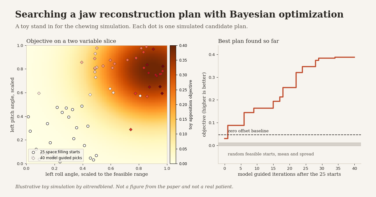
Read the numbers as plumbing checks and nothing more. The toy objective is smooth and has one hidden sweet spot, which makes the problem far easier than the real one. Still, two patterns mirror what the paper reports. The 25 space filling starts do not beat the zero offset baseline, with the best of them at 0.030 against a baseline of 0.047 and a random mean of 0.005, which is why the paper compares against both references. And after 40 model guided iterations the optimum reaches 0.387, with the safety regularized objective landing close behind at 0.369. In a run that we saved for the feature image, the best so far value first came within 5 percent of its final level at iteration 28 of 40 and within 1 percent at iteration 29. In the real problem each of those iterations costs about 6 minutes, which is why the acquisition rule matters.
What this adds up to
The core achievement is a working loop from a CT scan to a ranked set of surgical plans. A template based registration turns imaging into a personalized model of the jaw, muscles and joint. A chewing simulation scores a plan by how much donor bone stays in favorable contact with the native jaw. A Gaussian process with a sensible acquisition rule finds better plans in 75 evaluations. On three real patients the search beat the plan the surgeon delivered by up to 26 percentage points of mean apposition, and it beat random feasible plans by about a factor of three with a small spread between runs.
The conceptual shift is the more interesting part. Virtual surgical planning has long asked whether a reconstruction fits. This work asks whether it will load the joins in a way that bone tends to answer with growth. That is a change of question, from shape to mechanics, and it is forced by a fact the authors state plainly. Each patient has one realized plan, so the unrealized alternatives have no labels, and only a simulation can say anything about them.
The approach should travel, with changes. Anywhere a clinician picks among feasible alternatives that cannot all be tried, including implant alignment in orthopedics, radiotherapy beam arrangements and valve sizing, a personalized simulation plus a sample efficient optimizer is a plausible recipe. What would not travel unchanged is the surrogate. Apposition driven by strain energy is tuned to bone, and any other organ would need its own stand in that biology supports.
The remaining limitations are large and the authors list them. Three patients were optimized and four were checked against year 1 CT, with no outcome data on union or nonunion. The score is a comparative surrogate and leaves out vascularization, graft viability and fixation biology. The baseline is one surgeon’s plan per patient. The independent check, Dice overlap of 70.1 to 84.9 percent, comes without a chance level. Sensitivity was tested on material, contact and muscle parameters and not on the surrogate itself. None of this is hidden, and all of it limits what a reader should conclude.
The road ahead is laid out in the paper. The next steps are prospective evaluation in larger and more varied cohorts, surgeon preference studies and expert plan review, outcome studies with union and function endpoints, co optimization of plate geometry and screw placement along with the cut plane and donor variables, longer horizon healing models, intraoperative guidance, and priors learned from larger imaging cohorts. A fair test would also compare optimized plans with the unoptimized ones in a setting where a surgeon can rate them blind, because that measures something the simulation cannot grade for itself.
A surgical plan is a prediction about a year of healing, and this paper is an honest first attempt to put a number on it before the first cut is made.
Frequently asked questions
What is OsteoOpt++ and what does it do?
OsteoOpt++ is a research framework from Aftabi and colleagues that turns a pre operative CT into a patient specific digital twin of the jaw, muscles and joint, then uses Bayesian optimization to search six surgically controllable variables, such as cut plane angles and donor offsets, for mandibular reconstruction plans that keep donor bone in favorable contact with the native jaw.
Does it predict whether the bone will unite?
No. It scores each plan with a surrogate, the fraction of donor bone elements at the resection interface whose strain energy stimulus exceeds a remodeling threshold, averaged over a chewing cycle. The authors use it to compare candidate plans and say it does not model vascularization, graft viability, inflammation or long term healing.
How much better were the optimized plans?
Against the plan the surgeon actually implemented, cycle averaged donor mandible apposition rose by up to 26 percentage points in three real patients, and by up to 29 points against a common practice baseline on generic jaws. In Patient 1, for example, apposition rose from 10.3 percent for the surgeon baseline to 28.6 percent after optimization, while random feasible plans averaged 9.5 percent.
How was the prediction checked against real bone?
In four patients with day 5 and year 1 CT, predicted apposition was compared with bone formation seen at year 1. Dice overlap ranged from 70.1 to 84.9 percent and centroid differences from 0.24 to 1.82 mm. The paper presents this as consistency evidence for the surrogate and reports no union or nonunion outcome comparison.
How long does the planning take?
About 30 minutes of operator time per patient builds the digital twin once, and each optimization iteration takes about 6 minutes on a desktop with a consumer graphics card. Each run uses 75 evaluations, which the authors describe as a conservative cap. The workflow is meant for offline planning before surgery and not for use during the operation.
Can surgeons use it on patients today?
No. The paper describes a feasibility study using retrospective data from three optimization patients and four longitudinal patients, and its authors call for prospective evaluation in larger and more diverse cohorts. The authors’ code is public on GitHub as a research platform, and surgical decisions belong with the treating team.
Read the paper and explore the code
The article is open access under a Creative Commons Attribution license in Medical Image Analysis. The appendix holds the Gaussian process equations, the registration equations, the forward and inverse dynamics and the muscle parameter tables. The authors share the MATLAB workflow on GitHub and it needs ArtiSynth to run.
Aftabi, H., Lloyd, J. E., Ding, A., Sagl, B., Prisman, E., Hodgson, A., and Fels, S. Towards patient specific optimization for mandibular reconstruction planning based on predicted bone union propensity. Medical Image Analysis 115 (2027) 104281. DOI 10.1016/j.media.2026.104281. Open access, CC BY 4.0.
This analysis is based on the published paper and an independent evaluation of its claims.