
- Quantitative MRI
- Relaxometry
- Self supervised learning
- Physics guided deep learning
- MRI harmonization
- Brain imaging
- PyTorch
Picture a neuroradiologist who opens two brain scans of the same patient, one from spring and one from today. The patient is being followed after treatment for a brain tumor, and the scanner was replaced over the summer. The lesion looks a little brighter on the new T2 weighted image. Is that the tumor changing, or is it the machine? On ordinary MRI there is no number that settles it, because the picture depends on the scanner as much as on the tissue.
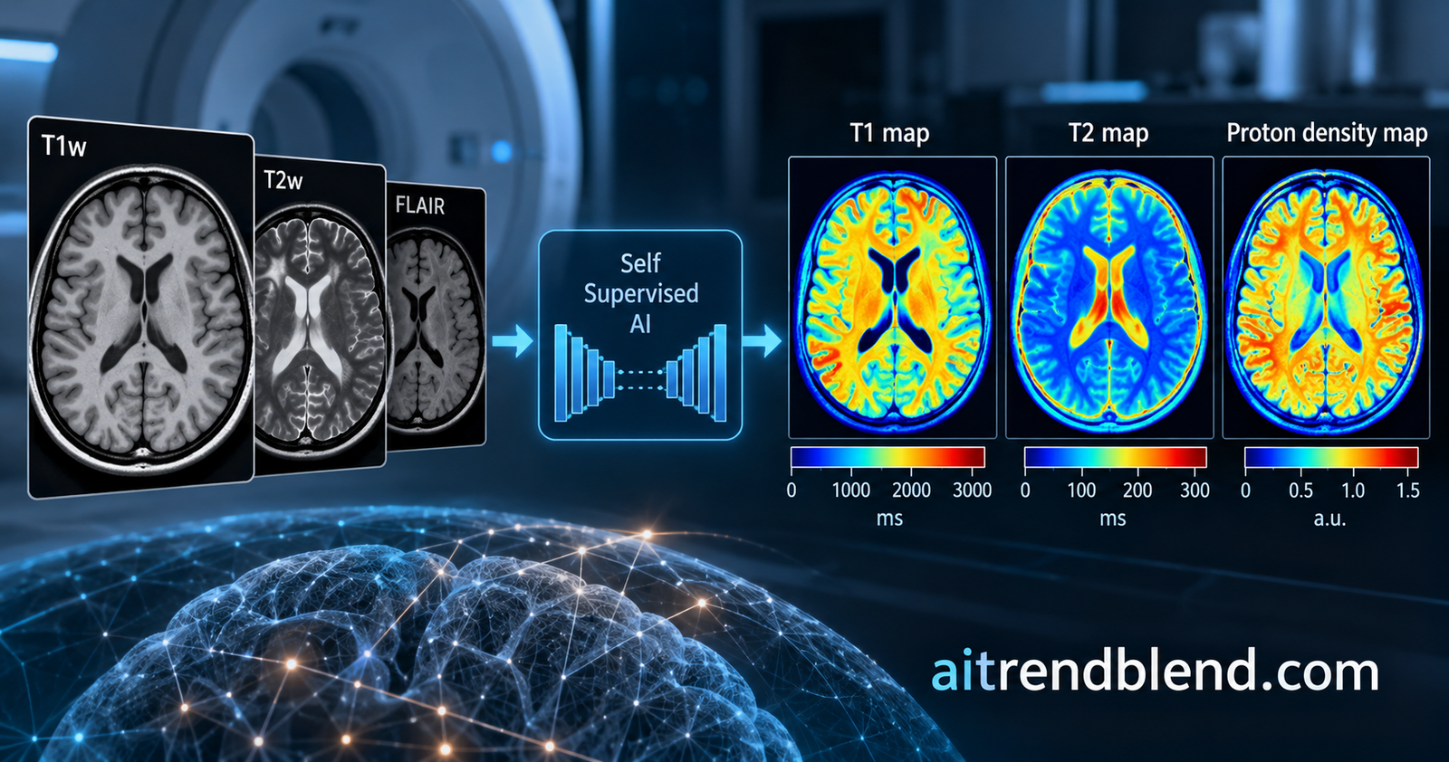
A group at University Medical Center Utrecht, led by Jelmer van Lune and Alessandro Sbrizzi, trained a network to turn exactly those ordinary scans into maps of T1, T2 and proton density, the physical properties of the tissue. They used 4121 clinical scan sessions and no reference maps at all. The work is open access in Medical Image Analysis and the code and weights are public. It is also careful about what it does not prove, which is where most of this article spends its time.
Key points
- The model reads routine T1 weighted, T2 weighted and FLAIR brain scans and outputs T1, T2 and proton density maps. It learns without any reference quantitative scan by forcing the maps to reproduce the input images through Bloch based signal equations.
- It was trained on 4121 sessions from 1786 subjects on four Philips 3 tesla scanners. On 603 held out sessions, white matter T1 averaged 834 ms and T2 averaged 69.1 ms, consistent with published ranges.
- Session averages barely moved across scanners or across nine groups of similar protocols. The inter group coefficient of variation stayed at or below 1.1 percent.
- In five people scanned twice, Pearson correlation and concordance exceeded 0.82 for T1 and T2 maps. T1 was the weaker map, with mean voxel wise differences of 6.9 to 14.8 percent.
- The maps were never checked against a dedicated quantitative sequence, every scanner in the test set was also in the training set, and the data come from one center and one vendor.
Medical disclaimer. This article explains a published research paper. It is not medical advice, diagnosis or treatment, and the maps described here are a research tool, not a clinical test. Any change seen on a brain scan needs interpretation by a qualified radiologist and treating clinician.
Why a brain scan is not a measurement
Ask what a T1 weighted image actually records and the honest answer is a tangle. The brightness of a voxel depends on intrinsic tissue properties, longitudinal relaxation time T1, transverse relaxation time T2 and proton density. It also depends on extrinsic choices, the scanner hardware, the vendor’s software, and sequence settings such as repetition time, echo time, inversion time and flip angle. Change any of them and the same tissue changes shade.
The paper is blunt about the consequences. Conventional MRI carries relative signal and no absolute meaning. That hinders longitudinal studies, makes objective biomarkers hard to build, and, as the authors point out (Wen and colleagues, 2023), degrades data driven image analysis models when the scanner changes.
Quantitative MRI, or qMRI, measures the underlying properties directly and would remove the ambiguity. Sequences such as MR fingerprinting (Ma and colleagues, 2013) shortened what used to be a very slow process, yet the paper notes that such sequences and their reconstruction tools are not widely available, especially outside academic hospitals. It then names a catch 22. Limited availability keeps the evidence thin, and thin evidence keeps hospitals from adopting the sequences (Hsieh and Svalbe, 2020).
So the field has tried to get quantitative maps out of the scans hospitals already have. Mathematical approaches need proton density weighted images, which modern clinical protocols rarely include, or rely on segmenting reference tissues (Moskovich and colleagues, 2024, and Wiltgen and colleagues, 2025). Supervised deep learning needs paired conventional and quantitative scans, and the paper argues such pairs are scarce and also biased, because each qMRI technique has its own sensitivities and no method is a universal gold standard (Bojorquez and colleagues, 2017).
Self supervised learning sidesteps the answer sheet. Earlier physics guided versions, including Qiu and colleagues (2024), showed the idea worked, but on small, clinically homogeneous datasets of tens to a few hundred subjects, mostly acquired with fixed protocols. Whether the idea survives a real hospital’s diversity was unanswered. The Utrecht team set out to test precisely that, and you can find related physics first thinking in our coverage of physics guided synthetic ultrasound and across the wider Medical AI archive.
Teaching a network physics without an answer sheet
Here is the trick in plain terms. The network looks at the three routine scans and proposes a T1 map, a T2 map and a proton density map. Then a set of physics equations, which know the exact repetition time, echo time, inversion time and flip angle of each scan, predict what each scan should look like if those maps were true. If the predicted images match the real ones, the maps are plausible. No one ever shows the network a correct map.
The equations come from Bloch physics for the three sequences in the dataset, a 3D spoiled gradient echo for T1 weighting, a 2D turbo spin echo for T2 weighting and a 3D turbo spin echo with inversion for FLAIR. The paper places its exact signal models in its supplement. The textbook forms below show their shape, and they are what our reconstruction in the code section uses.
Turbo spin echo sequences complicate the picture. They fire long trains of refocusing pulses with varying flip angles, so the effective T2 weighting differs from what the nominal echo time predicts. Following Busse and colleagues (2006), the authors adjust the nominal echo time with factors of 0.90 for the T2 weighted scans and 0.42 for FLAIR. That single number for FLAIR tells you how far a long echo train drifts from the textbook.
An ill posed puzzle
There is a snag the authors state directly. Turning three images into three maps is an inverse problem with many possible answers. Different combinations of T1, T2 and proton density can produce nearly the same pixel values, especially through the nonlinear exponentials above. Matching the input images is necessary and nowhere near sufficient.
So the training objective adds two guardrails to the image matching term. The first is total variation regularization, which discourages noisy, speckled maps. The second is a soft lower bound on proton density. Together with a scaling step described next, they form the whole loss.
The image term uses the L1 norm, so a few badly registered or artifact ridden voxels do not dominate. The final weights were 0.01 for total variation and 0.1 for the proton density bound. An ablation in the supplement, which the main text summarizes, removed each ingredient in turn. Dropping the global scaling constraint, the proton density bound, the total variation term or the contrast dropout either pushed values outside the literature ranges or reduced voxel wise reproducibility. The supplement carries the figures, so we cannot quote its numbers.
The scale problem hiding in plain sight
MRI scanners report intensities in arbitrary units, scaled by an unknown factor that changes from scan to scan. A physics model outputs signal in real units. To compare the two, something has to bridge the gap, and this is the least glamorous and arguably most important design decision in the paper.
First, every input volume is divided by the mode of its histogram, which corresponds to white matter. Then, for each subject and contrast, a scaling factor \(k\) is found in closed form by least squares, choosing the multiplier that best lines up the synthesized image with the real one.
If \(k\) were free, the network could cheat, since a proton density map that is twice as large with a scale factor half as large fits equally well. So \(k\) is constrained to stay within 20 percent of an analytic reference. That reference comes from the Bloch model evaluated on representative white matter values, proton density 0.70, T1 850 ms and T2 70 ms, together with each scan’s own sequence parameters.
Read that carefully. Absolute values are anchored by a prior about what white matter looks like. That is a sensible engineering choice, and the authors say it avoids needing any acquired reference qMRI. It also means the absolute numbers are not pure discoveries. The soft proton density bound sits at 0.60, and the reported white matter proton density is 0.59 with a standard deviation of 0.02, right at that threshold. That suggests, and this is our inference and not a statement in the paper, that the bound is probably active in white matter. A reader who treats the proton density map as a raw measurement should keep that in mind.
Self supervision removes the need for reference maps, and it does not remove the need for assumptions. Here the assumptions live in the scaling anchor, the proton density bound and the choice of signal model. They are reasonable, and they are also the reason absolute values deserve more caution than relative differences.
Inside the network
The model is a three level, 2D convolutional network shaped like a U Net (Ronneberger and colleagues, 2015). Two dimensions is a practical choice, because clinical T2 weighted scans use thick slices of 4 mm and the through plane resolution is much coarser than the in plane one. Each input slice is 224 by 224 pixels, and the output has three channels, one per map.
A shared weight encoder processes each contrast on its own. Every encoder level holds a residual block with two 3 by 3 convolutions, each followed by instance normalization and a ReLU, and downsampling uses a strided 3 by 3 convolution. Feature widths are 64, 128 and 256, and the bottleneck doubles that to 512. In total the network has about 8.6 million trainable parameters, and our reconstruction lands at 8.61 million, which is a useful sanity check on the layout.
The clever part sits between encoder and decoder. At every level, an attention module inspired by squeeze and excitation networks (Hu and colleagues, 2019) averages each contrast’s feature map, passes the summaries through a small shared two layer network, and turns the resulting scores into weights with a softmax across contrasts. The weighted features are then summed. The network can lean on the FLAIR features where they are informative and on the T1 weighted ones elsewhere, and it does so per level and per scan.
Because the encoder shares weights and the fusion is a softmax, the model does not care how many contrasts arrive. The authors exploit this during training with contrast dropout. Half of the time, one randomly chosen contrast is hidden from the network. That prevents over reliance on any single scan and, as an exploratory supplement figure suggests, helps when a contrast is missing at inference. Anyone following the missing scan problem will find a cousin of this idea in our article on missing modality medical imaging.
The decoder upsamples with transposed convolutions, concatenates the fused skip features, and refines with convolution blocks. A final 1 by 1 convolution produces three channels passed through a sigmoid. Those outputs are scaled linearly to physiological ranges, 0 to 1 for proton density, 0 to 5 seconds for T1 and 0 to 0.3 seconds for T2, which the authors say cover the full span of in vivo brain tissue values.
Training recipe
Training ran for 50 epochs with the Adam optimizer (Kingma and Ba, 2014), a learning rate of \(10^{-3}\), a batch of 16 slices and Kaiming initialization. Hyperparameters were tuned with Optuna, and model selection minimized validation loss while checking that outputs stayed inside physiologically expected ranges. The final weights came from the epoch with the lowest validation loss. Everything ran on a single NVIDIA Tesla V100 in about 30 hours with PyTorch 2.1.2, which puts it within reach of a well funded university lab and not only of a large industrial cluster.
A dataset that looks like a hospital
Scale and messiness are the paper’s real contribution. The team collected clinical scans from the radiology department at University Medical Center Utrecht between 2018 and 2023, covering the full range of neuro imaging protocols. They kept 3 tesla sessions that had a T1 weighted 3D spoiled gradient echo, a T2 weighted 2D turbo spin echo and a T2 FLAIR 3D turbo spin echo, the three most common contrasts in routine practice.
The result is 4121 sessions from 1786 unique subjects, aged 11 to 89 with a mean of 52.4 years and a standard deviation of 16.2. Of these, 54.9 percent were male and 45.1 percent female. Patients had oncology, neurodegenerative, epilepsy and vascular conditions among others, which is the point. Scans came from four Philips 3 tesla systems, Achieva at 34.1 percent, Ingenia at 27.5 percent, Ingenia CX at 21.8 percent and Ingenia Elition X at 16.6 percent.
The split was made by subject, about 80 percent for training, 5 percent for validation and 15 percent for testing. That gave 3312 training sessions from 1436 subjects, 206 validation sessions from 93 subjects, and 603 test sessions from 257 subjects.
| Parameter | T1w 3D spoiled GRE | T2w 2D TSE | T2 FLAIR 3D TSE |
|---|---|---|---|
| Gadolinium | No | Yes (98.1 percent) | Yes (35.9 percent) |
| TR (ms) | 5.03 to 5.40 | 3848 to 4557 | 4800 |
| TE (ms) | 2.247 to 2.493 | 80 | 280 to 370 |
| TI (ms) | not applicable | not applicable | 1650 |
| Flip angle (degrees) | 10 | 90 | 90 |
| Acquisition time | 1 min 59 s to 4 min 5 s | 54 s to 1 min 29 s | 3 min 17 s to 8 min 14 s |
Table 1. Sequence parameters of the clinical dataset, condensed from Table 1 of the paper.
Preprocessing was deliberately light. Scans were converted from DICOM, registered rigidly to the 2D T2 weighted image with ANTsPy, resampled to 1 by 1 mm in plane, cropped or padded to 224 by 224 and bias field corrected. Slices at the top and bottom of the head with low signal were dropped. There was no skull stripping and no tissue segmentation for the network input, unlike several earlier frameworks. Skull stripping and tissue segmentation appear only afterward, when white and gray matter masks, eroded by 2 mm away from cerebrospinal fluid to limit partial volume effects, are used to report numbers.
The gadolinium detail deserves a note. The T2 weighted scans were mostly acquired after contrast injection, and about a third of the FLAIR scans were as well. The authors kept them because contrast is usually given shortly beforehand and its effect on T2 weighting is minimal, though gadolinium shortens T1 and residual bias cannot be excluded. They excluded post contrast T1 weighted scans altogether.
What 603 test sessions show
For every test session the team computed the mean T1, T2 and proton density inside white matter and inside gray matter. Across all 603 sessions the distributions are stable and well separated. White matter T1 averaged 834 ms with a standard deviation of 37. Gray matter T1 averaged 1239 ms with a standard deviation of 50. The T2 values were 69.1 ms (standard deviation 1.0) for white matter and 89.5 ms (3.3) for gray matter. Proton density came out at 0.59 (0.02) and 0.65 (0.02).
| Tissue | T1 (ms) | T2 (ms) | PD (a.u.) |
|---|---|---|---|
| White matter | 834, SD 37 | 69.1, SD 1.0 | 0.59, SD 0.02 |
| Gray matter | 1239, SD 50 | 89.5, SD 3.3 | 0.65, SD 0.02 |
Table 2. Session level means across all 603 test sessions, quoted from the results section of the paper.
The authors judge these values consistent with literature reports (Bojorquez and colleagues, 2017, Stanisz and colleagues, 2005, and Choi and colleagues, 2022). That is a fair statement, and it is a weaker one than it sounds. Relaxation times vary considerably between measurement techniques, so a broad literature range is an easy target for any sensible model to hit. The stronger evidence comes next.
Do the maps care which scanner made the scan?
To test invariance the authors grouped the test sessions two ways. One grouping used the four scanner systems, with 189 sessions on Achieva, 164 on Ingenia, 125 on Ingenia Elition X and 125 on Ingenia CX. The other used nine protocol clusters found by agglomerative hierarchical clustering on the repetition and echo times of the three scans, with cluster sizes from 34 to 102 sessions. For each group they averaged the session means, then computed the coefficient of variation of those group means around the global mean.
| Grouping | T1 WM | T1 GM | T2 WM | T2 GM | PD WM | PD GM |
|---|---|---|---|---|---|---|
| Four scanner systems | 0.57 | 0.68 | 0.22 | 1.07 | 0.54 | 0.78 |
| Nine protocol clusters | 1.08 | 0.82 | 0.31 | 1.07 | 0.84 | 0.72 |
Table 3. Inter group coefficient of variation in percent, for white matter (WM) and gray matter (GM), quoted from the results section of the paper.
Every entry is at or below about 1.1 percent. The authors note this is lower than the repeatability reported for dedicated qMRI sequences scanned repeatedly in the same subject (Buonincontri and colleagues, 2019, and Liu and colleagues, 2025), and they conclude the maps are invariant to scanner hardware and protocol changes in their data.
We would read that with two qualifications. The first concerns the metric. A coefficient of variation of group averages measures how far the typical value shifts from group to group. With around a hundred sessions in a group, individual noise averages away, so the number is naturally small, and it is a different quantity from the scatter of individual sessions or from repeat scan differences in one person. The comparison with dedicated sequences therefore says less than the headline suggests.
The second concerns the test set. The split was made by subject, so every scanner and protocol in the test set also appeared in training. The result shows invariance across the scanners the model has seen, which is valuable for a hospital with a mixed fleet. It does not show that the model would behave on a scanner from another vendor or at another field strength. The authors say the same in their limitations, which we will come to.
What lesions look like on the maps
The paper also shows seven example patients, covering multiple sclerosis, a cavernous malformation, a meningioma and several gliomas, some after radiotherapy and chemotherapy. Compared with normal appearing white matter, the generated maps show prolongation of both T1 and T2 in lesions. T1 and T2 rose by 88.5 percent and 121.3 percent in the multiple sclerosis lesion, 83.1 percent and 89.8 percent in the meningioma, and 83.5 percent and 26.4 percent in the oligodendroglioma. The authors say these increases resemble those reported in the qMRI literature for these conditions, and that is an encouraging sign that the model keeps pathology visible instead of smoothing it toward the average.
Encouraging is the right word, and not more. Seven representative example slices are an illustration, and the paper reports no reader study or lesion classification test alongside them.
Same person, two scans
Invariance across groups is a statement about averages. A clinician wants to know whether one patient’s maps repeat. So the authors tested within subject reproducibility in five people, with three voxel wise metrics inside the brain parenchyma, Pearson correlation, the concordance correlation coefficient, and the mean voxel wise relative difference. The second scan was rigidly registered to the first before comparison.
Four subjects came from the clinical test set. Each had two sessions less than three months apart, no clinically relevant change in their lesions according to the neuroradiologist on the team, and good enough alignment. All four had brain lesions, and three were receiving treatment during the study, which adds real biological variation on top of any model error. Subject 1 had a diffuse astrocytoma treated with temozolomide, subject 2 had metastases from lung carcinoma and no treatment, subject 3 had melanoma metastases treated with nivolumab, and subject 4 had an anaplastic astrocytoma on temozolomide and anti epileptic medication. Subjects 2 to 4 were scanned on different scanners for their two sessions.
The fifth person was a healthy 26 year old volunteer, scanned twice back to back on one Philips Ingenia CX with two clinically representative protocols. They were chosen to sit at roughly the 20th and 80th percentiles of the dataset’s repetition and echo times. Nothing changed in the brain between those two scans, so this is the cleanest test in the paper.
| Subject | T1 r | T1 CCC | T1 diff | T2 r | T2 CCC | T2 diff | PD r | PD CCC | PD diff |
|---|---|---|---|---|---|---|---|---|---|
| 1 | 0.895 | 0.895 | 11.3% | 0.912 | 0.911 | 3.9% | 0.828 | 0.826 | 7.8% |
| 2 | 0.858 | 0.854 | 13.6% | 0.895 | 0.859 | 5.6% | 0.756 | 0.746 | 9.6% |
| 3 | 0.903 | 0.902 | 10.3% | 0.921 | 0.920 | 4.1% | 0.806 | 0.806 | 7.2% |
| 4 | 0.851 | 0.843 | 14.8% | 0.839 | 0.824 | 5.1% | 0.716 | 0.701 | 10.2% |
| Volunteer | 0.932 | 0.928 | 6.9% | 0.947 | 0.944 | 2.9% | 0.858 | 0.844 | 5.1% |
Table 4. Voxel wise within subject reproducibility, from Table 4 of the paper. The diff columns give the mean voxel wise relative difference.
The pattern is easy to read. T2 is the most reproducible map, with correlations from 0.839 to 0.947 and mean differences from 2.9 to 5.6 percent. T1 is next, with correlations from 0.851 to 0.932 but mean differences of 10.3 to 14.8 percent in the four patients and 6.9 percent in the volunteer. Proton density is the weakest, with correlations as low as 0.716. The abstract’s claim of excellent reproducibility, with Pearson and concordance exceeding 0.82, refers to T1 and T2, and proton density is not part of it.
Mean values in white and gray matter agree far better than individual voxels do. The largest difference in tissue means was 5.5 percent, for T1 in the white matter of subject 4. T2 white matter differences stayed under 2 percent in everyone, and the volunteer’s differences in means were under 2 percent for every parameter. So the maps are stable as regional averages and noisier voxel by voxel, as anyone would expect after registering two separate scans.
Why is T2 better than T1? The authors point to the inputs. The model sees two T2 weighted contrasts, T2w and FLAIR, and only one T1 weighted scan. They note this reverses a trend in the dedicated qMRI literature, where T1 usually reproduces better than T2. Gracien and colleagues (2020) reported voxel wise inter scanner differences up to 5.2 percent for T1 and T2 over intervals under five weeks, and Buonincontri and colleagues (2019) reported multi site coefficients of variation of 3 to 8 percent for T1, 8 to 14 percent for T2 and about 5 percent for proton density.
Compare them with care, since the metrics differ. A mean voxel wise relative difference and a coefficient of variation are different measurements, and the clinical subjects sat up to three months apart under treatment. Fair conclusions are narrower. The T2 map appears solid. The T1 map is usable for regional averages and noticeably noisier at voxel level. The paper’s own language, that findings are in line with the reported ranges for dedicated techniques, is more defensible than any claim of superiority.
“direct comparison with a reference qMRI method may obscure the model’s true performance.”van Lune and colleagues, Medical Image Analysis, 2027
Validation without a ground truth
The quote above captures a deliberate choice. Earlier self supervised and supervised studies mostly validated against an acquired reference qMRI scan. The authors argue that with no consensus technique and relaxation times that differ across methods, such a comparison would mostly measure disagreement between techniques. They chose to evaluate invariance and reproducibility instead, and they report the absolute values against literature ranges.
It is a defensible design, and it has a blind spot worth naming. Invariance is necessary for a good quantitative map and it is not sufficient. A network that painted every white matter voxel with 850 ms would be perfectly invariant across scanners and perfectly reproducible within subjects, and it would be useless. Two observations argue against that failure here. Voxel wise correlations between sessions reflect real anatomy, since a flat map would produce no correlation, and lesions show prolonged T1 and T2 values in the expected direction. Neither observation is the same as accuracy, which remains untested against any external reference in this paper.
The paper demonstrates that the maps are stable, that they are physiologically plausible and that they keep lesions visible. It does not demonstrate that a T1 of 834 ms in a given person is the true T1 of that person’s white matter. Use the maps for consistency across scanners and time, and treat absolute values as model outputs that carry priors.
The clinical translation gap
The authors frame the outlook around research. Because the method needs only routinely acquired T1 weighted, T2 weighted and FLAIR scans, no extra scan time is needed, and hospital archives could yield large scale studies of quantitative biomarkers. They mention brain tumor diagnosis and longitudinal monitoring, and neurodegenerative disease. That is a plan for biomarker research, and the paper stops short of clinical claims, with good reason.
Between these maps and a decision at the bedside sit several gaps. The paper offers no thresholds for what T1 or T2 value distinguishes one condition from another. It reports no reader study showing that a radiologist working with the maps decides better or faster than one working without them. And it has no data on how the maps behave on scanners, vendors or field strengths outside the training set. Any software that presented these maps as a diagnostic aid would in most jurisdictions face medical device regulation and would need that evidence. The paper reports no regulatory status and makes no such claim.
Transparency is a strength here. The authors publish code and trained weights on GitHub, so other groups can test the model on their own scanners. The patient data are confidential and cannot be shared. The work was funded by the Hanarth Fonds for AI in Oncology, and the authors declare no competing interests.
Where the model is known to be fragile
The discussion lists limits candidly. The Bloch signal models ignore factors such as transmit field inhomogeneity, magnetization transfer, partial volume effects and echo train dynamics. The T2 weighted and FLAIR scans that were acquired after gadolinium are kept, and while their effect is expected to be small, some residual bias cannot be excluded. Registering everything to the 2D T2 weighted geometry and resampling to 1 by 1 mm in plane costs through plane detail from the 3D scans, and slice thickness mismatches could complicate use in other centers.
The most practical warning concerns sequence types. A supplementary experiment found that when several sequence types for the same contrast were mixed during training, for example different flavors of T1 weighted acquisition, the resulting maps were not reproducible within subjects across those input types. In other words the model is safe within the sequence families it saw, and a hospital using inversion prepared gradient echo T1 weighting instead of spoiled gradient echo cannot assume the trained weights transfer. The authors point to richer signal models, extended phase graph formulations, explicit transmit field terms, or learning a more accurate model from data, as ways forward.
Where the idea could travel
If the approach holds up, the payoff is broader than better brain maps. Turning heterogeneous scans into a common quantitative space is a harmonization step, and the authors suggest it could make downstream deep learning models generalize better across sites. They also expect that the framework could extend to prostate and knee imaging, citing quantitative MRI work in those regions, though they only demonstrated brain data.
There is a pattern worth noticing across recent medical imaging work. Where labeled ground truth is missing, groups are replacing it with physics, either by simulating labeled data as in the synthetic ultrasound study or by making the network reproduce its own input through a forward model, as here. Self supervision through a forward model needs no simulator, and it inherits every simplification in the forward model. Our earlier look at tractography in pediatric epilepsy surgery shows the other side of brain imaging AI, where electrical stimulation mapping supplies a reference to learn from and to judge against.
Limitations, sample size and bias
Here are the constraints, using the paper’s own numbers.
- Reproducibility sample. Within subject reproducibility rests on five people, four patients with brain lesions and one healthy volunteer. Three of the four patients were under treatment, and the paper says larger dedicated datasets are needed.
- Single center and single vendor. All 4121 sessions came from one hospital and four Philips 3 tesla systems. The authors state that generalization to other sites, vendors and field strengths has not been established, and call cross site validation an important direction for future work.
- Test set overlap in scanners. The 603 test sessions were held out by subject, and every scanner and protocol also occurred in training. Invariance across unseen scanners is untested.
- No external reference. Accuracy was never compared with a dedicated qMRI acquisition, and absolute values rest partly on a white matter scaling anchor and a proton density bound at 0.60.
- T1 and proton density noise. Mean voxel wise differences reached 14.8 percent for T1 and 10.2 percent for proton density in the clinical subjects, and proton density correlations fell as low as 0.716.
- Sequence coverage. The model was built for three common Philips sequence types. Mixing other sequence types in training broke within subject reproducibility.
- Segmentation and registration. Tissue masks come from automatic segmentation that may be imperfect near lesions, and voxel wise comparisons depend on registration accuracy and partial volume effects.
- Clinical value unproven. No reader study, no diagnostic accuracy analysis and no outcome data accompany the maps.
None of this is hidden. The paper’s limitations section covers nearly every point above, which is a good sign of honest reporting and a useful checklist for anyone planning a follow up.
“This cross site validation remains an important direction for future work.”van Lune and colleagues, Medical Image Analysis, 2027
A PyTorch reconstruction of the framework
The authors released their own implementation, and anyone doing real work should start from their GitHub repository and trained weights. What follows is our independent reconstruction from the paper’s text, equations and Table 1 ranges, written to make every moving part visible in one file. The paper keeps its Bloch signal models in a supplement we did not have, so the signal equations are textbook forms and the comments mark every such choice as DESIGN CHOICE. This is educational code and it has never touched patient data.
The file holds the three signal models, the network with its shared encoder and attention fusion, the closed form global scaling, the three part loss, a training step with contrast dropout, the evaluation helpers for inter group coefficient of variation and within subject reproducibility, a phantom generator drawn from the Table 1 ranges, and a runnable smoke test. It needs Python 3, PyTorch 2 and NumPy.
"""
Self supervised, physics guided quantitative MRI mapping. Educational reference sketch.

Reconstructed from the description in
    van Lune et al. Quantitative mapping from conventional MRI using self supervised physics guided
    deep learning. Medical Image Analysis 115 (2027) 104295.  https://doi.org/10.1016/j.media.2026.104295
The authors publish their own code and weights at
    https://github.com/JelmervanL/Quantitative-mapping-from-conventional-MRI
Use that repository for real work. This file is an independent reconstruction written from the paper's
text, equations and Table 1 ranges. Where the paper leaves a detail open (the Bloch signal models sit in
its Supplementary Materials A, which we did not have) the comments say DESIGN CHOICE. It has not been
validated on patient data and it is not clinical software.

Layout
    1. Closed form signal models for T1w spoiled GRE, T2w TSE and T2 FLAIR
    2. Network, three level U Net like CNN, shared encoder, attention fusion across contrasts
    3. Global scaling, the three part loss (L1, total variation, proton density lower bound)
    4. Training step with contrast dropout and a fit loop
    5. Evaluation helpers, session means, inter group CV, within subject reproducibility
    6. A phantom generator and a runnable smoke test on dummy data
"""
import math
import numpy as np
import torch
import torch.nn as nn
import torch.nn.functional as F

CONTRASTS = ("T1w", "T2w", "FLAIR")          # channel order for inputs and synthesized images
MAP_NAMES = ("T1", "T2", "PD")               # channel order for the output maps
T1_MAX_S, T2_MAX_S, PD_MAX = 5.0, 0.3, 1.0   # sigmoid outputs are scaled to these ranges (Section 2.2.1)
TE_FACTOR = {"T2w": 0.90, "FLAIR": 0.42}     # TSE echo train corrections quoted in the paper
WM_REF = dict(pd=0.70, t1=0.850, t2=0.070)   # reference white matter values used for the scaling prior


# ---------------------------------------------------------------------------
# 1. Closed form signal models. All times in seconds, flip angle in radians.
# ---------------------------------------------------------------------------
def spoiled_gre(pd, t1, t2, tr, te, fa):
    """T1w 3D spoiled gradient echo. DESIGN CHOICE. Textbook steady state form with T2 decay at TE."""
    e1 = torch.exp(-tr / (t1 + 1e-6))
    return pd * torch.sin(fa) * (1 - e1) / (1 - torch.cos(fa) * e1 + 1e-6) * torch.exp(-te / (t2 + 1e-6))


def turbo_spin_echo(pd, t1, t2, tr, te):
    """T2w TSE. DESIGN CHOICE. Spin echo form, with the nominal TE scaled by the paper's correction."""
    te_eff = te * TE_FACTOR["T2w"]
    return pd * (1 - torch.exp(-tr / (t1 + 1e-6))) * torch.exp(-te_eff / (t2 + 1e-6))


def flair_tse(pd, t1, t2, tr, te, ti):
    """T2 FLAIR, inversion recovery turbo spin echo, magnitude image. DESIGN CHOICE as above."""
    te_eff = te * TE_FACTOR["FLAIR"]
    ir = 1 - 2 * torch.exp(-ti / (t1 + 1e-6)) + torch.exp(-tr / (t1 + 1e-6))
    return torch.abs(pd * torch.exp(-te_eff / (t2 + 1e-6)) * ir)


def synthesize(maps, seq):
    """maps  (B, 3, H, W) in the order T1 (s), T2 (s), PD (a.u.)
    seq   dict of per scan tensors shaped (B, 1, 1) for keys
          tr_t1w te_t1w fa_t1w   tr_t2w te_t2w   tr_fl te_fl ti_fl      (ms and degrees, as in the DICOM headers)
    returns (B, 3, H, W) synthesized T1w, T2w, FLAIR images before global scaling."""
    t1, t2, pd = maps[:, 0], maps[:, 1], maps[:, 2]
    ms = 1e-3
    a = spoiled_gre(pd, t1, t2, seq["tr_t1w"] * ms, seq["te_t1w"] * ms, torch.deg2rad(seq["fa_t1w"]))
    b = turbo_spin_echo(pd, t1, t2, seq["tr_t2w"] * ms, seq["te_t2w"] * ms)
    c = flair_tse(pd, t1, t2, seq["tr_fl"] * ms, seq["te_fl"] * ms, seq["ti_fl"] * ms)
    return torch.stack([a, b, c], dim=1)


def wm_reference_signal(seq):
    """Signal of the reference white matter (PD 0.70, T1 850 ms, T2 70 ms) for each contrast, shape (B, 3)."""
    ref = torch.tensor([WM_REF["t1"], WM_REF["t2"], WM_REF["pd"]]).view(1, 3, 1, 1)
    b = seq["tr_t1w"].shape[0]
    return synthesize(ref.expand(b, 3, 1, 1), seq).flatten(1)


# ---------------------------------------------------------------------------
# 2. Network. Shared weight encoder, softmax attention fusion, U Net decoder
# ---------------------------------------------------------------------------
class ConvINReLU(nn.Sequential):
    def __init__(self, cin, cout):
        super().__init__(nn.Conv2d(cin, cout, 3, padding=1), nn.InstanceNorm2d(cout, affine=True), nn.ReLU(inplace=True))


class ResBlock(nn.Module):
    """Residual block with two 3x3 conv, instance norm, ReLU units."""

    def __init__(self, cin, cout):
        super().__init__()
        self.body = nn.Sequential(ConvINReLU(cin, cout), ConvINReLU(cout, cout))
        self.skip = nn.Conv2d(cin, cout, 1) if cin != cout else nn.Identity()

    def forward(self, x):
        return self.body(x) + self.skip(x)


class AttentionFusion(nn.Module):
    """Squeeze and excitation style fusion across input contrasts.
    Global average pooling per contrast, a shared two layer MLP gives one logit per contrast, a softmax across
    contrasts turns them into weights, and the weighted feature maps are summed. It works for any number of
    inputs, and a boolean mask removes contrasts that are missing or dropped."""

    def __init__(self, channels, reduction=4):
        super().__init__()
        self.mlp = nn.Sequential(nn.Linear(channels, channels // reduction), nn.ReLU(inplace=True),
                                 nn.Linear(channels // reduction, 1))

    def forward(self, feats, present):
        # feats (B, N, C, H, W), present (B, N) boolean
        logits = self.mlp(feats.mean(dim=(-2, -1))).squeeze(-1)          # (B, N)
        logits = logits.masked_fill(~present, float("-inf"))
        w = torch.softmax(logits, dim=1)[:, :, None, None, None]
        return (w * feats).sum(dim=1), w[:, :, 0, 0, 0]          # fused features, attention weights (B, N)


class QMapNet(nn.Module):
    """Three level 2D U Net like CNN. Encoder widths 64, 128, 256, bottleneck 512, about 8.6 million weights."""

    def __init__(self, widths=(64, 128, 256), bottleneck=512):
        super().__init__()
        w1, w2, w3 = widths
        self.enc1, self.enc2, self.enc3 = ResBlock(1, w1), ResBlock(w1, w2), ResBlock(w2, w3)
        # DESIGN CHOICE. The strided 3x3 downsampling keeps the channel count, the next block widens it.
        self.down1 = nn.Conv2d(w1, w1, 3, stride=2, padding=1)
        self.down2 = nn.Conv2d(w2, w2, 3, stride=2, padding=1)
        self.down3 = nn.Conv2d(w3, w3, 3, stride=2, padding=1)
        self.bottleneck = nn.Sequential(ConvINReLU(w3, bottleneck), ConvINReLU(bottleneck, bottleneck))
        self.fuse1, self.fuse2, self.fuse3, self.fuse_b = (AttentionFusion(c) for c in (w1, w2, w3, bottleneck))
        self.up3 = nn.ConvTranspose2d(bottleneck, w3, 2, stride=2)
        self.up2 = nn.ConvTranspose2d(w3, w2, 2, stride=2)
        self.up1 = nn.ConvTranspose2d(w2, w1, 2, stride=2)
        self.dec3 = nn.Sequential(ConvINReLU(2 * w3, w3), ConvINReLU(w3, w3))
        self.dec2 = nn.Sequential(ConvINReLU(2 * w2, w2), ConvINReLU(w2, w2))
        self.dec1 = nn.Sequential(ConvINReLU(2 * w1, w1), ConvINReLU(w1, w1))
        self.head = nn.Conv2d(w1, 3, 1)
        for m in self.modules():                        # Kaiming initialisation, as in the paper
            if isinstance(m, (nn.Conv2d, nn.ConvTranspose2d, nn.Linear)):
                nn.init.kaiming_normal_(m.weight, nonlinearity="relu")
                if m.bias is not None:
                    nn.init.zeros_(m.bias)

    def forward(self, x, present=None):
        """x (B, 3, H, W) normalised T1w, T2w, FLAIR. present (B, 3) boolean, False for a dropped contrast.
        Returns maps (B, 3, H, W) in the order T1 (s), T2 (s), PD (a.u.)."""
        b, n, h, w = x.shape
        if present is None:
            present = torch.ones(b, n, dtype=torch.bool, device=x.device)
        x = x * present[:, :, None, None]                    # a dropped contrast is zeroed and ignored by fusion
        f1 = self.enc1(x.reshape(b * n, 1, h, w))            # shared weights, every contrast is one sample
        f2 = self.enc2(self.down1(f1))
        f3 = self.enc3(self.down2(f2))
        fb = self.bottleneck(self.down3(f3))
        split = lambda f: f.reshape(b, n, *f.shape[1:])
        s1, _ = self.fuse1(split(f1), present)
        s2, _ = self.fuse2(split(f2), present)
        s3, _ = self.fuse3(split(f3), present)
        sb, _ = self.fuse_b(split(fb), present)
        d3 = self.dec3(torch.cat([self.up3(sb), s3], dim=1))
        d2 = self.dec2(torch.cat([self.up2(d3), s2], dim=1))
        d1 = self.dec1(torch.cat([self.up1(d2), s1], dim=1))
        m = torch.sigmoid(self.head(d1))                     # (B, 3, H, W) in [0, 1]
        scale = torch.tensor([T1_MAX_S, T2_MAX_S, PD_MAX], device=x.device).view(1, 3, 1, 1)
        return m * scale


# ---------------------------------------------------------------------------
# 3. Global scaling and the three part loss
# ---------------------------------------------------------------------------
def histogram_mode_normalize(vol, mask, bins=100):
    """Divide a volume by the mode of its foreground histogram, which sits at the white matter intensity."""
    vals = vol[mask & (vol > 0)]
    hist, edges = np.histogram(vals, bins=bins)
    k = int(np.argmax(hist))
    return vol / (0.5 * (edges[k] + edges[k + 1]) + 1e-8)


def global_scale(img, synth, mask, k_ref, tol=0.2):
    """Eq. 1. Closed form least squares factor k = sum(I * I_hat) / sum(I_hat^2), then clamped to within
    plus or minus 20 percent of an analytic reference. img, synth (B, 3, H, W). mask (B, 1, H, W) float.
    k_ref (B, 3) is the reference factor. DESIGN CHOICE. Its direction follows Eq. 1, so k_ref = mode / S_WM."""
    num = (img * synth * mask).sum(dim=(-1, -2))
    den = (synth * synth * mask).sum(dim=(-1, -2)) + 1e-8
    k = num / den
    k = torch.minimum(torch.maximum(k, (1 - tol) * k_ref), (1 + tol) * k_ref)
    return k[:, :, None, None]


def total_variation(q, mask):
    """Eq. 3. Mean L2 norm of the spatial gradient, averaged over the three maps."""
    dx = F.pad(q[..., :, 1:] - q[..., :, :-1], (0, 1, 0, 0))
    dy = F.pad(q[..., 1:, :] - q[..., :-1, :], (0, 0, 0, 1))
    tv = torch.sqrt(dx ** 2 + dy ** 2 + 1e-12) * mask
    return tv.sum(dim=(-1, -2)).div(mask.sum(dim=(-1, -2)) + 1e-8).mean()


def pd_lower_bound(pd, mask, tau=0.60):
    """Eq. 4. Soft lower bound on PD, mean of max(0, tau - PD). DESIGN CHOICE. Only foreground voxels count."""
    return (torch.clamp(tau - pd, min=0) * mask[:, 0]).sum() / (mask.sum() + 1e-8)


def qmap_loss(maps, img, seq, mask, lambda_tv=0.01, lambda_pd=0.1):
    """Eq. 5. L = L_L1 + lambda_TV * L_TV + lambda_PD * L_PD.  Returns the total and its parts."""
    synth = synthesize(maps, seq)
    k_ref = 1.0 / (wm_reference_signal(seq) + 1e-8)          # normalised WM mode is 1, so k_ref = 1 / S_WM
    k = global_scale(img, synth, mask, k_ref)
    l1 = ((img - k * synth).abs() * mask).sum() / (mask.sum() * 3 + 1e-8)
    tv = total_variation(maps, mask)
    pdl = pd_lower_bound(maps[:, 2], mask)
    total = l1 + lambda_tv * tv + lambda_pd * pdl
    return total, {"l1": float(l1.detach()), "tv": float(tv.detach()), "pd": float(pdl.detach())}


# ---------------------------------------------------------------------------
# 4. Training with contrast dropout
# ---------------------------------------------------------------------------
def random_presence(batch, p_drop=0.5, device="cpu"):
    """Contrast dropout. With probability 0.5 one randomly chosen input contrast is omitted."""
    present = torch.ones(batch, 3, dtype=torch.bool, device=device)
    drop = torch.rand(batch, device=device) < p_drop
    which = torch.randint(0, 3, (batch,), device=device)
    present[torch.arange(batch, device=device)[drop], which[drop]] = False
    return present


def train_step(model, opt, img, seq, mask):
    """One optimisation step. The loss still compares all three synthesized images with all three real ones,
    so a dropped contrast must be inferred from the others. DESIGN CHOICE, the paper does not spell this out."""
    model.train()
    present = random_presence(img.shape[0], device=img.device)
    maps = model(img, present)
    loss, parts = qmap_loss(maps, img, seq, mask)
    opt.zero_grad()
    loss.backward()
    opt.step()
    return float(loss.detach()), parts


def fit(model, batches, epochs=50, lr=1e-3, log_every=0):
    """Adam with betas 0.9 and 0.999 and learning rate 1e-3, as in the paper. `batches` is a list of
    (img, seq, mask) tuples. The paper trains 50 epochs at batch size 16 and keeps the epoch with the lowest
    validation loss, and it tuned hyperparameters with Optuna. None of that tuning is repeated here."""
    opt = torch.optim.Adam(model.parameters(), lr=lr, betas=(0.9, 0.999))
    history = []
    for ep in range(epochs):
        losses = [train_step(model, opt, *b)[0] for b in batches]
        history.append(float(np.mean(losses)))
        if log_every and (ep % log_every == 0 or ep == epochs - 1):
            print(f"  epoch {ep:3d}  loss {history[-1]:.5f}")
    return history


# ---------------------------------------------------------------------------
# 5. Evaluation helpers
# ---------------------------------------------------------------------------
def session_mean(qmap, tissue_mask):
    """Mean of one quantitative map inside a tissue mask, for one scan session."""
    return float(qmap[tissue_mask].mean())


def inter_group_cv(session_means, group_ids):
    """Inter group coefficient of variation, as defined in Section 2.3.1. The standard deviation of the group
    means divided by the global mean, where a group mean averages its per session means and the global mean
    averages the group means. DESIGN CHOICE. Population standard deviation."""
    session_means, group_ids = np.asarray(session_means, float), np.asarray(group_ids)
    group_means = np.array([session_means[group_ids == g].mean() for g in np.unique(group_ids)])
    return float(group_means.std() / group_means.mean())


def reproducibility(a, b):
    """Voxel wise agreement between two sessions of the same subject. Returns Pearson r, Lin's concordance
    correlation coefficient and the mean voxel wise relative difference. DESIGN CHOICE. The relative difference
    is |a - b| divided by the pair mean, because the paper does not give the formula."""
    a, b = np.asarray(a, float).ravel(), np.asarray(b, float).ravel()
    r = float(np.corrcoef(a, b)[0, 1])
    ccc = float(2 * np.cov(a, b, bias=True)[0, 1] / (a.var() + b.var() + (a.mean() - b.mean()) ** 2))
    rel = float(np.mean(np.abs(a - b) / (0.5 * (a + b) + 1e-8)))
    return {"pearson_r": r, "ccc": ccc, "mean_rel_diff": rel}


# ---------------------------------------------------------------------------
# 6. Phantom and smoke test
# ---------------------------------------------------------------------------
TISSUES = {  # (T1 s, T2 s, PD). DESIGN CHOICE. Round values, CSF kept inside the network's output range.
    "wm": (0.850, 0.070, 0.70), "gm": (1.240, 0.090, 0.65), "csf": (3.500, 0.300, 1.00), "lesion": (1.600, 0.140, 0.85)}


def make_phantom(size=64, seed=0):
    """A small head shaped phantom with white matter, gray matter, ventricles and one lesion.
    Returns true maps (3, H, W) as T1, T2, PD, a brain mask, and a dict of tissue masks."""
    rng = np.random.default_rng(seed)
    yy, xx = np.mgrid[:size, :size]
    cy, cx = size / 2 + rng.uniform(-1, 1), size / 2 + rng.uniform(-1, 1)
    r = np.sqrt(((yy - cy) / (0.46 * size)) ** 2 + ((xx - cx) / (0.38 * size)) ** 2)
    brain, wm = r < 1.0, r < 0.78
    vent = (np.abs(yy - cy) < 0.10 * size) & (np.abs(xx - cx) < 0.16 * size) & wm
    lesion = ((yy - cy - 0.22 * size) ** 2 + (xx - cx + 0.16 * size) ** 2) < (0.07 * size) ** 2
    lesion &= wm
    lab = {"gm": brain & ~wm, "wm": wm & ~vent & ~lesion, "csf": vent, "lesion": lesion}
    maps = np.zeros((3, size, size), np.float32)
    for name, m in lab.items():
        for c in range(3):
            maps[c][m] = TISSUES[name][c]
    return torch.from_numpy(maps), brain, lab


def random_sequence(batch, rng):
    """Sequence parameters drawn inside the Table 1 ranges of the paper (ms and degrees)."""
    u = lambda lo, hi: torch.tensor(rng.uniform(lo, hi, (batch, 1, 1)), dtype=torch.float32)
    return {"tr_t1w": u(5.03, 5.40), "te_t1w": u(2.247, 2.493), "fa_t1w": torch.full((batch, 1, 1), 10.0),
            "tr_t2w": u(3848, 4557), "te_t2w": torch.full((batch, 1, 1), 80.0),
            "tr_fl": torch.full((batch, 1, 1), 4800.0), "te_fl": u(280, 370), "ti_fl": torch.full((batch, 1, 1), 1650.0)}


def make_batch(batch, size, rng, noise=0.01):
    """Phantom scans with unknown global scale, then histogram mode normalisation as in preprocessing."""
    maps, imgs, masks = [], [], []
    for i in range(batch):
        q, brain, _ = make_phantom(size, seed=int(rng.integers(1e6)))
        maps.append(q)
        masks.append(torch.from_numpy(brain.astype(np.float32)))
    maps, masks = torch.stack(maps), torch.stack(masks)[:, None]
    seq = random_sequence(batch, rng)
    with torch.no_grad():
        raw = synthesize(maps, seq) * torch.tensor(rng.uniform(200, 900, (batch, 3, 1, 1)), dtype=torch.float32)
    raw = raw + noise * raw.max() * torch.randn_like(raw) * masks
    for i in range(batch):
        for c in range(3):
            raw[i, c] = torch.from_numpy(
                histogram_mode_normalize(raw[i, c].numpy(), masks[i, 0].numpy().astype(bool))).float()
    return raw * masks, seq, masks, maps


def smoke_test(steps=25, size=64, batch=4):
    """Runs end to end on dummy data. It confirms the parameter count, the shapes, that the loss falls,
    that a dropped contrast still yields maps, and that the evaluation helpers compute. It does NOT
    show quantitative accuracy, and 25 steps is nothing next to 50 epochs on 3312 sessions."""
    torch.manual_seed(0)
    rng = np.random.default_rng(0)
    model = QMapNet()
    n_params = sum(p.numel() for p in model.parameters())
    print(f"trainable parameters {n_params / 1e6:.2f} million (paper reports about 8.6 million)")

    img, seq, mask, truth = make_batch(batch, size, rng)
    maps = model(img)
    assert maps.shape == (batch, 3, size, size)
    assert (maps[:, 0] <= T1_MAX_S).all() and (maps[:, 1] <= T2_MAX_S).all() and (maps[:, 2] <= PD_MAX).all()
    dropped = torch.tensor([[True, False, True]] * batch)
    assert torch.isfinite(model(img, dropped)).all(), "dropped contrast broke the forward pass"

    opt = torch.optim.Adam(model.parameters(), lr=1e-3)
    losses = []
    for s in range(steps):
        loss, parts = train_step(model, opt, img, seq, mask)
        losses.append(loss)
        if s % 5 == 0 or s == steps - 1:
            print(f"  step {s:3d}  loss {loss:.4f}  l1 {parts['l1']:.4f}  tv {parts['tv']:.4f}  pd {parts['pd']:.4f}")
    assert np.isfinite(losses).all() and losses[-1] < losses[0], "loss did not fall"

    # Evaluation helpers on dummy session means and dummy voxel values.
    sess = np.concatenate([rng.normal(834, 30, 40), rng.normal(830, 30, 40), rng.normal(838, 30, 40)])
    groups = np.repeat([0, 1, 2], 40)
    cv = inter_group_cv(sess, groups)
    a = rng.normal(1200, 200, 5000)
    rep = reproducibility(a, a + rng.normal(0, 60, 5000))
    print(f"dummy inter group CV {100 * cv:.2f} percent   dummy reproducibility r {rep['pearson_r']:.3f}  "
          f"CCC {rep['ccc']:.3f}  mean rel diff {100 * rep['mean_rel_diff']:.1f} percent")
    print("smoke test passed")


if __name__ == "__main__":
    smoke_test()
The smoke test checks plumbing. It confirms the parameter count, the output shapes and ranges, that a dropped contrast still yields finite maps, that the loss falls on phantom data, and that the evaluation helpers compute. The last line uses random numbers, so it describes the helper functions and nothing else.
The parameter count of 8.61 million matches the paper’s figure of about 8.6 million, which is a good sign that the layout is faithful. The loss curve says nothing about accuracy, because 25 steps is nothing next to 50 epochs on 3312 sessions. In a separate 200 step run on random phantoms, the white matter T2 came back at 0.0695 s against a true 0.070 s, proton density at 0.65 against 0.70, and T1 far too low, at 0.52 s against a true 0.85 s. It is a toy run with a toy loop, and it does fit the ill posed picture the paper describes, in which T1 is the map the constraints have the hardest time pinning down.
Where this leaves us
The core achievement is easy to state. A network trained on 4121 clinical sessions, with no reference maps, turned routine T1 weighted, T2 weighted and FLAIR scans into T1, T2 and proton density maps whose tissue averages barely changed across four scanners and nine protocol groups, with inter group coefficients of variation at or below 1.1 percent. That is a much harder setting than the small, homogeneous datasets earlier self supervised work used, and it holds up.
The conceptual shift matters as much as the numbers. Conventional MRI has always been read as pictures. This work treats each scan as the output of a physical forward model and asks the network to run it backwards, with the scanner settings supplied as knowns. The picture and the settings together become a measurement. The engineering around it, the scale anchor, the proton density bound and the contrast dropout, shows how much careful design lies between an elegant idea and maps that stay inside physiological ranges.
The idea should travel where a trustworthy forward model exists and reference data are scarce. Harmonizing archives from mixed scanner fleets, tracking lesions across scanner upgrades, and feeding stable inputs to downstream models are all natural uses, and the authors mention prostate and knee as next candidates. Two lessons carry over to any field. Self supervision through a forward model inherits every simplification of that model, and invariance is easier to demonstrate than accuracy.
The remaining limitations are real and the authors list them. The data come from one center and four Philips scanners, all of which also appear in training. Within subject checks cover five people, T1 and proton density are noisier than T2 at voxel level, no dedicated qMRI acquisition was used as a reference, and mixing sequence types in training broke reproducibility. Absolute values rest partly on a white matter anchor and a proton density bound, so relative comparisons deserve more trust than raw numbers.
The road ahead is clear from the discussion. The next steps are validation across sites, vendors and field strengths, richer signal models that include transmit field effects and magnetization transfer, support for more sequence types, larger reproducibility cohorts, and above all a test against a dedicated quantitative sequence and against clinical outcomes. Public code and weights mean other groups can begin that work now, and the first useful result from any of them will be a held out scanner the model has never seen.
An MRI scan has always been a photograph taken by a particular machine. This paper makes a serious, honest case that it can also be a measurement, and it is honest enough to say how much of that case still has to be proved.
Frequently asked questions
What does this model produce from a routine brain MRI?
It produces quantitative T1, T2 and proton density maps from three routine scans, a T1 weighted 3D spoiled gradient echo, a T2 weighted 2D turbo spin echo and a T2 FLAIR 3D turbo spin echo. No extra scan time is needed, and no dedicated quantitative sequence was used for training.
How does the network learn without reference quantitative maps?
It is trained with self supervision. The predicted maps are passed through Bloch based signal models that use each scan’s repetition time, echo time, inversion time and flip angle, and the synthesized images are compared with the real scans using an L1 loss. Total variation regularization, a soft lower bound on proton density and a constrained global scaling step keep the ill posed problem in check.
How consistent are the maps across scanners and protocols?
On 603 held out sessions, the inter group coefficient of variation across four Philips 3 tesla scanners was between 0.22 and 1.07 percent, and across nine protocol clusters it was between 0.31 and 1.08 percent. White matter averaged 834 ms for T1 and 69.1 ms for T2. Every test scanner also appeared in training, so unseen scanners remain untested.
Are the quantitative values accurate?
The paper does not compare them with a dedicated quantitative MRI acquisition. It shows that values fall within published literature ranges and that they reproduce within subjects, with Pearson and concordance correlations above 0.82 for T1 and T2 in five people. Accuracy against an external reference remains untested.
Will it work on other scanners or other sequence types?
That has not been shown. All data came from one center and four Philips 3 tesla systems, and a supplementary experiment found that mixing several sequence types for the same contrast during training made maps less reproducible within subjects. The authors identify cross site validation as an important direction for future work.
Can these maps be used for clinical decisions today?
No. The paper positions the maps for research on quantitative biomarkers and reports no reader study, diagnostic thresholds or outcome data. The code and trained weights are public on GitHub, and any clinical interpretation of a brain scan belongs with a qualified radiologist and treating clinician.
Read the paper and run the code
The article is open access under a Creative Commons Attribution license in Medical Image Analysis. The supplement holds the signal model equations, the ablation study, the sequence type experiment and extra reproducibility figures. The authors share code and trained weights on GitHub.
van Lune, J., Mandija, S., van der Heide, O., Maspero, M., Schilder, M. B., Dankbaar, J. W., van den Berg, C. A. T., and Sbrizzi, A. Quantitative mapping from conventional MRI using self supervised physics guided deep learning, Applications to a large scale, clinically heterogeneous dataset. Medical Image Analysis 115 (2027) 104295. DOI 10.1016/j.media.2026.104295. Open access, CC BY 4.0.
This analysis is based on the published paper and an independent evaluation of its claims.