
- Random forests
- Ensemble weighting
- Fractional gradients
- Caputo derivative
- Model selection
- UCI benchmarks
- PyTorch
A fraud analyst at a bank trains a random forest of a hundred trees on card transactions. Some of those trees happen to be excellent at spotting one rare kind of fraud and mediocre at everything else. Others are the reverse. When a new transaction arrives, every tree casts one vote with equal weight, and the specialist’s insight about the rare class gets drowned out by ninety nine generalists.
A team of researchers from Algeria, Saudi Arabia, Turkey, India, Cyprus, the United Arab Emirates and France proposes a fix with two parts. Give each tree a separate, learned weight for each class it votes on. Then tune those weights with a gradient step that borrows its shape from fractional calculus, so that every weight’s recent history shapes how far it moves next.
Key points
- fCWRFO replaces the single vote of each tree with a matrix of tree by class weights, trained by softmax cross entropy on top of a fixed random forest.
- A fractional order \(\alpha\) rescales each weight’s gradient step using the range that weight has visited so far. At \(\alpha = 1\) this is ordinary gradient descent.
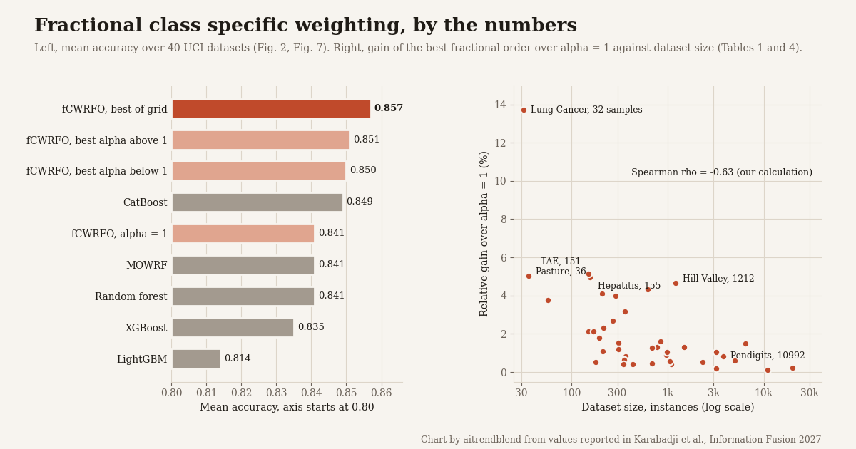
- Across 40 UCI datasets the best fractional order gives a mean accuracy of 0.857, ahead of CatBoost at 0.849 and random forest at 0.841, with significant Wilcoxon results against all five baselines.
- With \(\alpha = 1\), the weighted forest averages 0.841, the same as a plain random forest. The whole gain comes from choosing the best of eleven fractional orders for each dataset.
- That choice is made on the reported cross validated accuracy, and the gain is largest on the smallest datasets, which calls for caution before reading it as a general improvement.
Why equal votes waste expertise
Leo Breiman’s random forest, introduced in 2001, remains one of the most dependable tools in machine learning. Grow many decision trees, each on a bootstrap sample of the data with a random subset of features at every split, and let them vote. The randomness decorrelates the trees, and averaging decorrelated trees reduces variance without adding much bias. On tabular data with a few hundred to a few hundred thousand rows, a forest with default settings is often hard to beat.
The voting rule, though, is blunt. Every tree gets one vote, whatever its quality and whatever the class. Researchers have chipped at this for two decades. Early work weighted trees by out of bag accuracy. Later approaches learned one global weight per tree through convex optimization, including an optimal weighted forest analyzed by Chen, Yu and Zhang in the Journal of Machine Learning Research in 2024. Class based coefficients and heuristic reweighting schemes followed. Most of these still give each tree a single number, which assumes a tree is equally good or equally bad at every class.
That assumption rarely holds. A tree that split early on a feature that separates class A from everything else will be sharp on class A and noisy on B and C. The authors, led by Nour Elislem Karabadji of the National Higher School of Technology and Engineering in Annaba, Algeria, with Ahmed Al Nuaim of King Faisal University and Wajdi Dhifli of Université de Lille as corresponding authors, have worked on weighted and pruned forests before, and this paper, Fractional class specific weighted random forest optimization, published in Information Fusion, takes the idea to the finest grain available, a weight for every pair of tree and class.
The problem of choosing fusion weights shows up far outside forests. Our analysis of why equal weighted hyperspectral anomaly fusion fails reaches a similar conclusion in a very different setting. Equal weights are a default, not an answer.
A weight for every tree and every class
The construction is clean. Train an ordinary random forest with \(N\) trees. For each training sample \(j\), record which class each tree predicts as a one hot vector \(O^{(t)}_{j,c}\). Introduce a weight matrix \(W\) of size \(N \times C\), initialized to \(1/N\), and form weighted logits with a Bernoulli dropout mask \(m_t\) that randomly silences some trees during training.
The trees themselves are frozen. Only \(W\) is learned. Because the logits are linear in \(W\) and the loss is softmax cross entropy, the problem is convex in the weights, just like multinomial logistic regression on fixed features. The gradient has a tidy form. For each weight it is the average prediction error on class \(c\), counted only over samples where tree \(t\) voted for \(c\).
The paper walks through a worked example with three trees and two classes. Logits of 0.9 and 1.4 give probabilities of 0.378 and 0.622 and a loss of about 0.475 when the true class is the second one. A standard step with learning rate 0.1 then lowers the weight of every tree that voted for the wrong class by 0.0378 and raises the weight of every tree that voted for the right one by the same amount. After each step the weights are projected back into the interval from 0 to 1, which keeps them interpretable as confidence scores.
That is the whole class specific part. It is sensible, cheap and easy to implement. The second part is where the paper’s name comes from.
What fractional means here
Fractional calculus generalizes derivatives to non integer orders. The Caputo derivative of order \(\alpha\) between 0 and 1 is an integral over the function’s past, weighted by a power law kernel, so it carries memory of where the function has been rather than only its slope at a single point.
The authors apply this idea to each weight separately. The lower terminal \(\mu_{t,c}\) is the smallest value that weight has taken so far, and a matching right sided derivative uses the largest value \(\nu_{t,c}\). Computing these integrals exactly would require the loss gradient at every point along the interval, which is impractical. So they approximate the gradient as constant over the interval, which collapses both integrals into closed form and absorbs the Gamma factor into the learning rate. What remains is the ordinary gradient multiplied by a scaling factor.
When \(\alpha = 1\), the exponent is zero, \(\Psi = 1\), and the update is plain gradient descent. When \(\alpha\) is below 1, \(\Psi\) depends on how far the weight sits from the edges of the range it has explored. The paper’s third example shows a weight at 0.9 near the top of a range from 0 to 1 getting \(\Psi \approx 0.633\), so its step shrinks from 0.038 to 0.024, while a weight at 0.6 in the middle gets \(\Psi \approx 0.704\). The authors describe this as a history dependent diagonal preconditioner, which is the most useful way to think about it.
The paper is careful here, and deserves credit for it. It calls the practical update a Caputo inspired first order approximation, states that the approximation error is of order \(h^{2-\alpha}\) where \(h\) is the local interval length, and notes that extending the scheme to orders between 1 and 2, which it tests empirically, is a formal extension of the scaling rule rather than a new Caputo derivation. The convergence theorem is proved only for \(\alpha\) between 0 and 1.
The convergence guarantee
Under Lipschitz smoothness of the loss with constant \(L\), and with \(\Psi\) bounded between \(\psi_{\min}\) and \(\psi_{\max}\) thanks to the stabilizer \(\varepsilon\) and the projection onto the unit interval, the authors show through the descent lemma that the loss is monotonically non increasing and the gradient goes to zero whenever the learning rate satisfies a simple bound.
This is the standard analysis for preconditioned gradient descent with a bounded diagonal preconditioner, and it goes through as expected. Two practical caveats apply. The proof treats the update as unconstrained, while the algorithm projects the weights and applies random tree dropout at every step. And the experiments fix the learning rate at 0.1 across all datasets and orders without checking it against the bound. Neither undermines the method, but the theorem describes an idealized version of what runs.
Stripped of the calculus, fCWRFO is multinomial logistic regression on frozen tree votes, trained with a per weight step size that depends on how much of its range each weight has explored. The fractional order controls the shape of that step size schedule.
A practical reading of the fractional order
Here is where it gets interesting. Consider the very first iteration. Every weight starts at \(1/N\), so its historical minimum and maximum equal its current value, and both terms in \(\Psi\) reduce to \(\varepsilon^{1-\alpha}\). The step size at the start is therefore \(\eta\,\varepsilon^{1-\alpha}\).
If \(\varepsilon\) is small, the consequences are large. With \(\varepsilon = 0.01\), an order of 0.5 shrinks the initial step by a factor of 10, while an order of 1.3 enlarges it by a factor of almost 4, as our code prints below. Orders below 1 start cautiously and speed up as each weight explores its range. Orders above 1 start aggressively and slow down. Because the experiments hold the base learning rate at 0.1 and the budget at 100 epochs with early stopping for every dataset, choosing \(\alpha\) is partly choosing an effective learning rate schedule for each dataset.
That is not a criticism of the idea. Adaptive, history aware step sizes are exactly what methods like Adagrad and Adam provide, and a well chosen schedule can matter a lot. But it changes what a comparison between \(\alpha = 1\) and the best \(\alpha\) actually measures. It would have been informative to compare against plain gradient descent with its own learning rate tuned over an eleven value grid. The paper does not report the value of \(\varepsilon\), so the size of this effect in its experiments cannot be pinned down from the text.
The observation also fits a finding the paper reports without dwelling on. On the Balance Scale dataset the optimal order of 1.3 converged in 11.4 epochs on average against 16.5 for the integer baseline. A larger effective step early on would produce exactly that.
What the numbers say
The evaluation uses 40 UCI datasets, from Lung Cancer with 32 samples to Letter with 20,000, and from 2 to 26 classes. Everything runs under stratified 10 fold cross validation with a fixed seed. The weights train for at most 100 epochs with learning rate 0.1, an L2 penalty of 0.01 and early stopping after 20 epochs without improvement. The baselines are a scikit-learn random forest with 100 trees, XGBoost, CatBoost, LightGBM and the authors’ own multiobjective weighted random forest, MOWRF, all with default hyperparameters.
fCWRFO is evaluated at eleven orders, 0.1, 0.3, 0.5, 0.7, 0.9, 1.0, 1.1, 1.3, 1.5, 1.7 and 1.9. The reported score for each dataset is the maximum accuracy over this grid.
| Method | Mean accuracy |
|---|---|
| fCWRFO, best order per dataset | 0.857 |
| fCWRFO, best order above 1 per dataset | 0.851 |
| fCWRFO, best order below 1 per dataset | 0.850 |
| CatBoost | 0.849 |
| MOWRF | 0.841 |
| Random forest | 0.841 |
| fCWRFO, order fixed at 1.0 | 0.841 |
| XGBoost | 0.835 |
| LightGBM | 0.814 |
Mean over 40 UCI datasets, from Fig. 2 and Fig. 7 of the paper.
The best order per dataset produced the best or tied best accuracy on 21 of 40 datasets, and a strictly best result on 17. The Wilcoxon signed rank tests below compare these per dataset maxima with each baseline.
| fCWRFO versus | Wins / ties / losses | z score | p value |
|---|---|---|---|
| Random forest | 36 / 4 / 0 | minus 5.45 | 5.08 × 10⁻⁸ |
| MOWRF | 33 / 1 / 6 | minus 4.49 | 7.11 × 10⁻⁶ |
| XGBoost | 29 / 5 / 6 | minus 4.33 | 1.46 × 10⁻⁵ |
| LightGBM | 28 / 0 / 12 | minus 3.76 | 7.71 × 10⁻⁵ |
| CatBoost | 24 / 3 / 13 | minus 2.14 | 0.033 |
Table 3 of the paper.
No dataset picked \(\alpha = 1\) as its best order. Eighteen chose an order below 1 and twenty two chose an order above 1, with 1.3 the most common choice on 13 datasets and 0.1 next on 7. Every dataset reached its best displayed accuracy at some non integer order.
How to read a best of grid result
The numbers tell a complicated story, and it rewards a careful read. The table above contains the key fact. With the order fixed at 1.0, the class specific weighted forest averages 0.841, exactly the same as the plain forest it is built on. The weighting scheme alone, under the paper’s protocol, does not improve accuracy on average. Every point of the gain over random forest, from 0.841 to 0.857, comes from choosing the best of eleven orders for each dataset.
The paper defines the reported estimator as the maximum over the order grid of the cross validated accuracy, and it does not describe a nested step in which the order is selected on data separate from the folds used for scoring. When you pick the best of eleven noisy estimates, the maximum is biased upward even if the eleven configurations are equally good. The bias grows as the estimates get noisier, and cross validated accuracy on a dataset with a few dozen samples is very noisy.
The paper’s own table points the same way. The largest relative gains over the integer order appear on Lung Cancer, with 32 samples, at 13.73 percent, then TAE with 151 samples, Pasture with 36, Hepatitis with 155 and Hill Valley with 1212. The smallest, 0.10 percent, is on Pendigits with nearly 11,000 samples. On Lung Cancer, the move from 0.517 to 0.588 amounts to a little over two correctly classified patients out of 32. We computed the rank correlation between dataset size and gain across all 40 datasets from Tables 1 and 4, and it comes out at minus 0.63. The median gain is 3.0 percent on the twelve datasets with fewer than 250 samples and 0.6 percent on the twelve with 1000 or more.
We also tested the effect directly on six small datasets available offline. Using the implementation below, the paper’s grid maximum averaged 0.896, while a nested version that picks the order on an inner validation split and scores it on the untouched test fold averaged 0.886, slightly below plain random forest at 0.894. Six datasets settle nothing, and our weights are fitted on out of bag votes, a choice the paper does not specify, so our absolute numbers will not match theirs. The direction, though, is what one would expect from selection optimism.
The Wilcoxon tests inherit the same issue. Each compares one tuned configuration, the best of eleven, against baselines run with defaults and no tuning at all. That is why the comparison with random forest can show 36 wins and no losses even though the \(\alpha = 1\) version of the same model ties it on average. LightGBM’s weak average also reflects defaults poorly suited to tiny datasets. It scores 0.283 on Pasture, 0.400 on Lung Cancer and 0.647 on Labor, datasets with 36, 32 and 57 samples, where its default leaf size constraints leave little room to split.
The fair comparison is fCWRFO with an order chosen inside each training fold against baselines with an equal tuning budget. Until that comparison is run, the 1.6 point average gain should be read as an upper bound that includes model selection on the reported accuracy.
“These results indicate that different datasets benefit from different degrees of adaptive gradient scaling. Thus, the order α acts as a tunable optimization and regularization parameter.”Karabadji and colleagues, Information Fusion, 2027
That is the reading the paper itself supports, and it is a reasonable one. The fractional order is a hyperparameter. Hyperparameters need to be chosen without looking at the test data.
Memory direction, dropout and sparsity
Left, right or both
The scaling factor has two halves, one measured from the historical minimum and one from the historical maximum. The authors compared each half alone with the two sided average on four datasets at orders between 0.7 and 0.9. Neither half wins everywhere. The left sided version acts as a strong regularizer on Waveform 5000 and Breast Cancer, where the integer order model overfits after about 40 epochs, but it stagnates on TAE and Glass, where the right sided version converges and the left does not. The two sided average avoids both failure modes, which is why it is the default. This part of the study rests on accuracy curves from four datasets, so it is best read as guidance rather than proof.
Tree dropout
Randomly masking trees during weight training, with drop rates from 0 to 0.5, gives smooth loss curves on larger datasets such as Waveform 5000 even at a rate of 0.3. On small datasets such as Glass and TAE, rates of 0.4 and above make the loss visibly jagged, although it stays bounded. The dropout rate used in the main benchmark is not stated alongside the other hyperparameters.
Keeping only the strongest classes per tree
A Top K variant keeps, for each tree, only its \(K\) largest class weights and zeroes the rest. This turns the weight matrix into an explicit map of which trees act as experts for which classes.
| Configuration | Eligible datasets | Dense accuracy | Sparse accuracy | Links removed | W / T / L | p value |
|---|---|---|---|---|---|---|
| Top 1 | 40 | 0.8570 | 0.8474 | 66.57% | 10 / 2 / 28 | 0.0042 |
| Top 2 | 23 | 0.8620 | 0.8543 | 57.62% | 3 / 4 / 16 | 0.0062 |
| Top 3 | 13 | 0.8714 | 0.8656 | 64.46% | 2 / 0 / 11 | 0.0159 |
| Top 5 | 12 | 0.8800 | 0.8784 | 46.25% | 3 / 1 / 8 | 0.2477 |
| Top 10 | 4 | 0.9263 | 0.9280 | 37.83% | 2 / 0 / 2 | 0.7150 |
Table 5 of the paper. Each row covers only datasets with more classes than K, so rows are not directly comparable.
Aggressive sparsity costs accuracy significantly. Top 5 removes nearly half of all tree class links with a drop of only 0.16 points that is not significant. The authors are explicit that this is about interpretability, not speed, since the implementation still uses dense matrices.
Cost
Weight optimization is cheap next to growing the forest. Across three synthetic scenarios, the optimization step adds 7.2 percent to forest construction time at 10,000 samples, 2.4 percent at 50,000 and 1.3 percent at 100,000. With 100 classes it takes 3.08 seconds against 241.47 seconds to build the forest. The fractional scaling itself adds essentially nothing. Running at an order of 0.5 took between 0.93 and 1.10 times as long as running at 1.0 across sample sizes from 10,000 to 100,000. Complexity per epoch is dominated by the forward pass over samples, trees and classes, and the fractional power operations touch only the \(N \times C\) weights.
Limitations
Order selection. The reported accuracy is a maximum over an eleven value grid of cross validated scores, without a described nested selection step. Gains concentrate on the smallest datasets, where this kind of selection is least reliable. The paper names adaptive, self regulated fractional orders as its first direction for future work, which would remove the grid search altogether.
Tuning asymmetry. All baselines run with defaults, while fCWRFO has its order tuned per dataset. The integer order version, which receives no such tuning, matches random forest on average.
Theory versus practice. The convergence proof covers orders between 0 and 1 and an unconstrained update. The experiments use orders up to 1.9, projection onto the unit interval and random tree dropout. The stabilizer value, which controls the initial step size, is not reported.
Unspecified details. The paper does not state on which samples the weights are fitted. Trees predict their own bootstrap samples almost perfectly, so fitting on in bag predictions rewards memorization, while fitting on out of bag votes or a held out split avoids it. The dropout rate for the main benchmark and the size of the internal validation split are also not given.
Reproducibility. The paper states that data will be made available on request, and we found no code release. The UCI datasets are public, but reproducing the exact numbers requires rebuilding the pipeline.
Minor inconsistencies. The text attributes a gain of 4.97 percent to Heart Statlog, while Table 4 lists that figure for Hepatitis and 2.69 percent for Heart Statlog. The text states that a 500 tree ensemble needs 2.58 seconds of optimization, while the corresponding figure shows about one second. Neither changes the conclusions.
Who should care
For practitioners with tabular data, the class specific weighting is worth trying on its own, independent of the fractional machinery. It is a cheap post processing step on an existing forest, it can be fitted on out of bag votes so no extra data is needed, and the Top K variant yields a readable map of which trees specialize in which classes. That map can be useful in domains such as fraud, where the analyst cares about one rare class, a setting our coverage of online anomaly detection under concept drift also explores.
For researchers in optimization, the paper is a clear example of a fractional order method reduced to what it does in practice, a bounded, history dependent diagonal preconditioner. That framing makes it comparable with the adaptive methods already in wide use, and it suggests the experiments that would isolate its contribution. Our pieces on how biased stochastic gradients still generalize and on pruning and generalization theory look at related questions from the neural network side, and the optimization and learning theory archive collects more.
For anyone reading benchmark papers, the lesson is about protocol. When a method has a hyperparameter the baselines lack, and the reported score is the best value over a grid, the first number to look for is the method’s score with that hyperparameter fixed. Here it was printed in the paper, and it tells the most honest part of the story.
Reference implementation in PyTorch
The code below implements the full method in one file. It builds one hot tree votes from a fitted scikit-learn random forest, initializes the tree by class weight matrix to \(1/N\), and forms the weighted logits with Bernoulli tree dropout. It computes the softmax cross entropy and its closed form gradient, tracks the historical minimum and maximum of every weight, and applies the two sided, left or right fractional scaling. The update is projected onto the unit interval with the paper’s learning rate, L2 penalty, epoch budget and early stopping patience. Top K sparsification, an experts per class count and the full evaluation protocol with the eleven value order grid and the Wilcoxon test are included too.
Two choices the paper leaves open are made explicit. Weights are fitted on out of bag votes by default, and the evaluation reports both the paper’s grid maximum and a nested estimate in which the order is chosen inside each training fold. For Top K, the mask is taken from the dense solution and the retained weights are refined again, because a mask taken at the uniform initialization would be arbitrary. The smoke test reproduces the paper’s three worked examples, prints the initial scaling factor for two orders, and runs both protocols on six small datasets that ship with scikit-learn.
"""
fCWRFO, Fractional Class-Specific Weighted Random Forest Optimization.
Reference implementation of
    Karabadji, Lakhdari, Al Nuaim, Algefary, Yildirim, Assi, Elati, Dhifli.
    Fractional class-specific weighted random forest optimization.
    Information Fusion 138 (2027) 104689. https://doi.org/10.1016/j.inffus.2026.104689

What is implemented
    * one hot tree votes O (J x N x C) from a fitted scikit-learn random forest
    * the class specific weight matrix W (N x C) initialised to 1/N (Algorithm 1)
    * weighted logits z_jc = sum_t m_t W_tc O_jtc with Bernoulli tree dropout m_t (Eq. 6)
    * softmax cross entropy (Eq. 7-8) and its closed form gradient (Eq. 9, 13)
    * the Caputo inspired fractional scaling Psi from the historical extrema of every weight,
      two sided (Eq. 15), plus the left sided and right sided variants of Sec. 5.4.4
    * projected update W <- clip(W - eta * Psi * grad, 0, 1) (Eq. 12, 14)
    * L2 penalty 0.01, eta 0.1, 100 epochs, early stopping with patience 20 (Sec. 5.1)
    * tree level Top-K sparsification (Eq. 19-22)
    * the evaluation protocol, stratified 10 fold CV, an alpha grid, and the Wilcoxon test

Choices the paper does not specify, marked "our choice" below
    * which samples W is fitted on. Trees predict their own bootstrap samples almost perfectly,
      so by default we fit W on out of bag votes only (each tree contributes to a training sample
      only when that sample was out of its bootstrap). Set weight_data="train" for in-bag votes.
    * the stabiliser epsilon and the size of the internal validation split used for early stopping
    * alpha selection. The paper reports max over the alpha grid of the cross validated accuracy.
      We implement that ("oracle") and a nested variant that picks alpha on an inner validation
      split of each training fold, so the optimism of grid maximisation can be measured.
"""
import math
import numpy as np
import torch
from scipy.stats import wilcoxon
from sklearn.ensemble import RandomForestClassifier
from sklearn.model_selection import StratifiedKFold, train_test_split

ALPHA_GRID = (0.1, 0.3, 0.5, 0.7, 0.9, 1.0, 1.1, 1.3, 1.5, 1.7, 1.9)

# ---------------------------------------------------------------------------
# 1. Tree votes
# ---------------------------------------------------------------------------

def tree_votes(forest, X, n_classes):
    """One hot votes O[j, t, c] = 1 if tree t predicts class c for sample j (Sec. 4.1)."""
    preds = np.stack([est.predict(X).astype(int) for est in forest.estimators_], 1)   # (J, N)
    O = np.zeros((X.shape[0], len(forest.estimators_), n_classes), dtype=np.float32)
    np.put_along_axis(O, preds[..., None], 1.0, axis=2)
    return torch.from_numpy(O)


def oob_mask(forest, n_samples):
    """A[j, t] = 1 if sample j was out of tree t's bootstrap sample."""
    A = np.ones((n_samples, len(forest.estimators_)), dtype=np.float32)
    for t, idx in enumerate(forest.estimators_samples_):
        A[np.unique(idx), t] = 0.0
    return torch.from_numpy(A)

# ---------------------------------------------------------------------------
# 2. The fractional optimizer for W
# ---------------------------------------------------------------------------

class FractionalScaler:
    """Tracks mu (historical min) and nu (historical max) of every weight and returns
        two sided  Psi = ((w - mu + eps)^(1-a) + (nu - w + eps)^(1-a)) / 2      (Eq. 15)
        left       Psi = (w - mu + eps)^(1-a)
        right      Psi = (nu - w + eps)^(1-a)
    alpha = 1 gives Psi = 1 and recovers plain gradient descent."""

    def __init__(self, W0, alpha, eps=1e-2, mode="two"):
        self.mu, self.nu = W0.clone(), W0.clone()
        self.alpha, self.eps, self.mode = alpha, eps, mode

    def update_history(self, W):
        self.mu = torch.minimum(self.mu, W)
        self.nu = torch.maximum(self.nu, W)

    def psi(self, W):
        if self.alpha == 1.0:
            return torch.ones_like(W)
        e = 1.0 - self.alpha
        left = (W - self.mu + self.eps).clamp(min=1e-12) ** e
        right = (self.nu - W + self.eps).clamp(min=1e-12) ** e
        return {"two": 0.5 * (left + right), "left": left, "right": right}[self.mode]


def logits(W, O, mask_tree, avail=None):
    """z_jc = sum_t m_t * a_jt * W_tc * O_jtc. `avail` is the out of bag availability (our choice)."""
    M = mask_tree[None, :] if avail is None else mask_tree[None, :] * avail
    return torch.einsum("jt,tc,jtc->jc", M, W, O)


def ce_and_grad(W, O, Y1h, mask_tree, avail=None, l2=0.01):
    """Softmax cross entropy (Eq. 8) and its gradient dL/dW_tc = 1/J sum_j (P_jc - y_jc) m_t O_jtc (Eq. 9)."""
    z = logits(W, O, mask_tree, avail)
    P = torch.softmax(z, 1)
    loss = -(Y1h * torch.log(P.clamp(min=1e-12))).sum(1).mean() + 0.5 * l2 * (W ** 2).sum()
    M = mask_tree[None, :] if avail is None else mask_tree[None, :] * avail
    grad = torch.einsum("jc,jt,jtc->tc", P - Y1h, M, O) / O.shape[0] + l2 * W
    return loss, grad


class FCWRFO:
    def __init__(self, n_trees=100, alpha=1.0, eta=0.1, epochs=100, l2=0.01, p_drop=0.1, patience=20,
                 eps=1e-2, mode="two", top_k=None, weight_data="oob", val_frac=0.2, seed=42):
        self.n_trees, self.alpha, self.eta, self.epochs, self.l2 = n_trees, alpha, eta, epochs, l2
        self.p_drop, self.patience, self.eps, self.mode, self.top_k = p_drop, patience, eps, mode, top_k
        self.weight_data, self.val_frac, self.seed = weight_data, val_frac, seed

    # ---- forest ------------------------------------------------------------
    def fit_forest(self, X, y):
        self.classes_ = np.unique(y)
        self.C = len(self.classes_)
        self.enc = {c: i for i, c in enumerate(self.classes_)}
        yi = np.array([self.enc[v] for v in y])
        self.forest = RandomForestClassifier(n_estimators=self.n_trees, random_state=self.seed).fit(X, yi)
        self.O_train = tree_votes(self.forest, X, self.C)
        self.avail = oob_mask(self.forest, len(X)) if self.weight_data == "oob" else None
        self.y_train = yi
        return self

    # ---- Top-K sparsification (Eq. 19-20) ------------------------------------
    def topk_mask(self, W):
        if self.top_k is None or self.top_k >= self.C:
            return torch.ones_like(W)
        idx = W.abs().topk(self.top_k, dim=1).indices
        return torch.zeros_like(W).scatter_(1, idx, 1.0)

    # ---- weight optimisation (Algorithm 1) -----------------------------------
    def _optimize(self, W, K, alpha, O_tr, Y_tr, A_tr, O_va, Y_va, A_va, g, record):
        scaler = FractionalScaler(W, alpha, self.eps, self.mode)
        best, best_W, wait, hist = float("inf"), W.clone(), 0, []
        ones = torch.ones(self.n_trees)
        epoch = -1
        for epoch in range(self.epochs):
            m = (torch.rand(self.n_trees, generator=g) >= self.p_drop).float()   # m_t ~ Bernoulli(1 - p_drop)
            loss, grad = ce_and_grad(W * K, O_tr, Y_tr, m, A_tr, self.l2)
            W = (W - self.eta * scaler.psi(W) * grad * K).clamp(0.0, 1.0)       # Eq. 12, 14 and projection
            scaler.update_history(W)
            val_loss, _ = ce_and_grad(W * K, O_va, Y_va, ones, A_va, 0.0)
            if record:
                hist.append((loss.item(), val_loss.item()))
            if val_loss.item() < best - 1e-6:
                best, best_W, wait = val_loss.item(), W.clone(), 0
            else:
                wait += 1
                if wait >= self.patience:
                    break
        return best_W * K, epoch + 1, hist

    def fit_weights(self, alpha=None, train_idx=None, val_idx=None, record=False):
        """Dense optimisation of W. With top_k set, the Top-K mask is taken from the dense solution
        and the retained tree class weights are optimised again with the mask fixed (our reading
        of Sec. 5.6, a mask taken at the uniform initialisation would be arbitrary)."""
        alpha = self.alpha if alpha is None else alpha
        g = torch.Generator().manual_seed(self.seed)
        n = len(self.y_train)
        if train_idx is None:
            train_idx, val_idx = train_test_split(np.arange(n), test_size=self.val_frac,
                                                  stratify=self.y_train, random_state=self.seed)
        O_tr, O_va = self.O_train[train_idx], self.O_train[val_idx]
        A_tr = None if self.avail is None else self.avail[train_idx]
        A_va = None if self.avail is None else self.avail[val_idx]
        Y_tr = torch.nn.functional.one_hot(torch.as_tensor(self.y_train[train_idx]), self.C).float()
        Y_va = torch.nn.functional.one_hot(torch.as_tensor(self.y_train[val_idx]), self.C).float()
        args = (O_tr, Y_tr, A_tr, O_va, Y_va, A_va, g, record)
        W0 = torch.full((self.n_trees, self.C), 1.0 / self.n_trees)
        W, self.epochs_run, self.history = self._optimize(W0, torch.ones_like(W0), alpha, *args)
        if self.top_k is not None and self.top_k < self.C:
            K = self.topk_mask(W)
            W, ep, _ = self._optimize(W * K, K, alpha, *args)
            self.epochs_run += ep
        self.W = W
        return self

    def fit(self, X, y):
        return self.fit_forest(X, y).fit_weights()

    # ---- inference -----------------------------------------------------------
    def predict_proba(self, X):
        O = tree_votes(self.forest, X, self.C)
        return torch.softmax(logits(self.W, O, torch.ones(self.n_trees)), 1).numpy()

    def predict(self, X):
        return self.classes_[self.predict_proba(X).argmax(1)]

    def experts_per_class(self):
        """E_c = number of trees that keep class c among their Top-K weights (Eq. 22)."""
        return (self.W > 0).sum(0).numpy()

# ---------------------------------------------------------------------------
# 3. Evaluation protocol
# ---------------------------------------------------------------------------

def evaluate_dataset(X, y, alphas=ALPHA_GRID, folds=10, seed=42, **kw):
    """Stratified CV. For every fold, the forest is fitted once and W is refitted for every alpha.
    Returns accuracies of plain RF, of each alpha, the paper's grid maximum ("oracle"), and a
    nested estimate where alpha is chosen on an inner validation split of the training fold."""
    skf = StratifiedKFold(folds, shuffle=True, random_state=seed)
    acc_rf, acc_alpha, acc_nested = [], {a: [] for a in alphas}, []
    for tr, te in skf.split(X, y):
        model = FCWRFO(seed=seed, **kw).fit_forest(X[tr], y[tr])
        acc_rf.append((model.forest.predict(X[te]) == np.array([model.enc.get(v, -1) for v in y[te]])).mean())
        inner_tr, inner_va = train_test_split(np.arange(len(tr)), test_size=0.2, stratify=y[tr], random_state=seed)
        inner_scores = {}
        for a in alphas:
            model.fit_weights(alpha=a, train_idx=inner_tr, val_idx=inner_va)
            acc_alpha[a].append((model.predict(X[te]) == y[te]).mean())
            O_va = model.O_train[inner_va]
            p = logits(model.W, O_va, torch.ones(model.n_trees)).argmax(1).numpy()
            inner_scores[a] = (p == model.y_train[inner_va]).mean()
        a_star = max(alphas, key=lambda a: (inner_scores[a], -abs(a - 1.0)))
        acc_nested.append(acc_alpha[a_star][-1])
    per_alpha = {a: float(np.mean(v)) for a, v in acc_alpha.items()}
    best_alpha = max(per_alpha, key=per_alpha.get)
    return dict(rf=float(np.mean(acc_rf)), per_alpha=per_alpha, oracle=per_alpha[best_alpha],
                best_alpha=best_alpha, nested=float(np.mean(acc_nested)))


def wilcoxon_report(a, b):
    """Wins, ties, losses and the two sided Wilcoxon signed rank p value for paired accuracies."""
    d = np.round(np.asarray(a) - np.asarray(b), 6)
    w, t, l = int((d > 0).sum()), int((d == 0).sum()), int((d < 0).sum())
    p = wilcoxon(d[d != 0]).pvalue if (d != 0).sum() > 0 else 1.0
    return w, t, l, round(float(p), 4)

# ---------------------------------------------------------------------------
# 4. Smoke test
# ---------------------------------------------------------------------------

def worked_examples():
    """Reproduce Examples 1 to 3 of the paper by hand."""
    z = np.array([0.9, 1.4])
    P = np.exp(z) / np.exp(z).sum()
    print(f"Example 1, P = {P.round(3)}, loss = {-np.log(P[1]):.3f}      paper 0.378, 0.622, 0.475")
    g = P - np.array([0, 1])
    print(f"Example 2, integer updates {(-0.1 * g).round(4)}               paper -0.0378, +0.0378")
    for w, gg, name in [(0.9, g[0], "Case A"), (0.6, g[1], "Case B")]:
        psi = (math.sqrt(w - 0) + math.sqrt(1 - w)) / 2
        print(f"Example 3 {name}, Psi = {psi:.3f}, new w = {w - 0.1 * psi * gg:.3f}")
    print("                                      paper Case A 0.633, 0.876   Case B 0.704, 0.627")


if __name__ == "__main__":
    from sklearn.datasets import load_breast_cancer, load_wine, load_iris, load_digits, make_classification
    torch.manual_seed(0)
    worked_examples()

    # (a) Psi at the first iteration, when the history interval is still empty
    for a in (0.5, 1.3):
        print(f"Psi at iteration 0 with eps 1e-2, alpha {a}: {(1e-2) ** (1 - a):.3f}")

    # (b) Grid maximum versus nested alpha selection on six datasets
    datasets = {
        "breast cancer": load_breast_cancer(return_X_y=True),
        "wine": load_wine(return_X_y=True),
        "iris": load_iris(return_X_y=True),
        "digits (subset)": tuple(a[:600] for a in load_digits(return_X_y=True)),
        "synthetic 3 class": make_classification(300, 20, n_informative=6, n_classes=3, flip_y=0.1, random_state=1),
        "synthetic small": make_classification(60, 10, n_informative=4, n_classes=2, flip_y=0.1, random_state=2),
    }
    rows = []
    print(f"\n{'dataset':18s} {'RF':>6s} {'a=1.0':>6s} {'grid max':>8s} {'best a':>6s} {'nested':>7s}")
    for name, (X, y) in datasets.items():
        r = evaluate_dataset(X, y, n_trees=100, p_drop=0.1)
        rows.append(r)
        print(f"{name:18s} {r['rf']:6.3f} {r['per_alpha'][1.0]:6.3f} {r['oracle']:8.3f} {r['best_alpha']:6.1f} {r['nested']:7.3f}")
    mean = lambda k: np.mean([r[k] for r in rows])
    print(f"{'average':18s} {mean('rf'):6.3f} {np.mean([r['per_alpha'][1.0] for r in rows]):6.3f} {mean('oracle'):8.3f} {'':6s} {mean('nested'):7.3f}")
    print("grid max vs RF   W/T/L and p:", wilcoxon_report([r["oracle"] for r in rows], [r["rf"] for r in rows]))
    print("nested vs RF     W/T/L and p:", wilcoxon_report([r["nested"] for r in rows], [r["rf"] for r in rows]))

    # (c) Top-K sparsification and memory orientation on one dataset
    X, y = load_wine(return_X_y=True)
    Xtr, Xte, ytr, yte = train_test_split(X, y, test_size=0.3, stratify=y, random_state=0)
    for k in (None, 1, 2):
        for mode in ("two", "left", "right"):
            m = FCWRFO(alpha=0.7, top_k=k, mode=mode).fit(Xtr, ytr)
            acc = (m.predict(Xte) == yte).mean()
            print(f"wine hold out, top_k {str(k):4s} mode {mode:5s} acc {acc:.3f} epochs {m.epochs_run:3d} "
                  f"experts per class {m.experts_per_class().tolist()}")
Running the file on a laptop CPU takes a few minutes and prints the following. The worked examples match the paper up to rounding in the last digit. The dataset rows show the grid maximum above the nested estimate on average. With six datasets, none of the Wilcoxon results is meaningful as a test, and they are printed to show the machinery works.
Conclusion
Karabadji and colleagues start from a real weakness in random forests. Equal voting ignores the fact that trees specialize, and a single weight per tree cannot capture specialization by class. Their answer, a learned weight for every tree and class trained by softmax cross entropy on frozen votes, is simple, convex, cheap to fit and easy to add to any existing forest. The Top K analysis shows that nearly half of those weights can be removed without a significant loss, leaving an interpretable map of which trees serve which classes.
The fractional part reframes gradient descent through the Caputo derivative and, after a careful first order approximation, arrives at a per weight scaling factor based on how much of its range each weight has explored. The paper is admirably precise about what that approximation is and is not, and it proves convergence for orders below one under standard assumptions. Seen plainly, the result is a history dependent diagonal preconditioner, a close relative of the adaptive optimizers used throughout deep learning.
The idea travels. Any ensemble with fixed base learners, from boosting stages to model soups to mixtures of classifiers, could learn class specific combination weights the same way. Fractional or history aware step size scaling could be tested against Adam and Adagrad on any convex problem with bounded parameters, which would show whether the power law form adds something beyond adaptivity.
The limits sit mostly in the evaluation. With the order fixed at one, the weighted forest ties plain random forest on average. The reported gains come from choosing the best of eleven orders per dataset on the scored accuracy, they are largest on the smallest and noisiest datasets, and they are compared against baselines that received no tuning. The initial step size depends on a stabilizer whose value is not reported, and the theory covers a simpler update than the one that runs.
The next experiments are clear. Select the order inside each training fold, give the baselines an equal tuning budget, compare against plain gradient descent with a tuned learning rate, and release the code. If the fractional scaling still helps after that, it will have earned its place. The class specific weighting may prove the more lasting contribution either way, because a forest that knows which of its trees to trust for which class is a better forest.
Frequently asked questions
What is fCWRFO?
fCWRFO, the Fractional Class Specific Weighted Random Forest, is a method that learns a separate weight for every pair of tree and class in a trained random forest. The weights are fitted with softmax cross entropy on the trees’ fixed votes, using a gradient step rescaled by a fractional order that depends on each weight’s history.
How is class specific weighting different from weighting trees?
Ordinary weighted forests give each tree one number, which assumes a tree is equally reliable for every class. Class specific weighting gives each tree one number per class, so a tree that is sharp on one class and noisy on others can be trusted only where it performs well.
What does the fractional order alpha do?
It rescales the gradient step for each weight based on how far that weight sits from the smallest and largest values it has taken so far. At alpha equal to 1 the method is ordinary gradient descent. Values below 1 start with small steps, and values above 1 start with larger steps, so alpha acts as a history dependent step size control.
How much does fCWRFO improve accuracy?
On 40 UCI datasets, choosing the best of eleven fractional orders per dataset gives a mean accuracy of 0.857, against 0.849 for CatBoost and 0.841 for random forest. With alpha fixed at 1, the method averages 0.841, the same as random forest, so the gain depends on selecting alpha per dataset.
Is the comparison with XGBoost and CatBoost fair?
Only partly. The fractional order is tuned per dataset by taking the best of eleven values on the reported accuracy, while the boosting baselines use default hyperparameters. A fairer test would choose alpha inside each training fold and give the baselines an equal tuning budget.
Does fCWRFO slow down a random forest?
Very little. The weight optimization adds about 7.2 percent to forest construction time at 10,000 samples and 1.3 percent at 100,000, and the fractional scaling itself costs almost nothing compared with ordinary gradient descent.
Read the full paper
The article is open access under a Creative Commons Attribution license in Information Fusion, with the full derivation, the convergence proof, per dataset results for all eleven fractional orders and the sparsification and runtime studies.
Karabadji, N. E., Lakhdari, A., Al Nuaim, A., Algefary, A., Yildirim, Y., Assi, A., Elati, M., and Dhifli, W. Fractional class specific weighted random forest optimization. Information Fusion 138 (2027) 104689. DOI 10.1016/j.inffus.2026.104689.
This analysis is based on the published paper and an independent evaluation of its claims.