
Key points
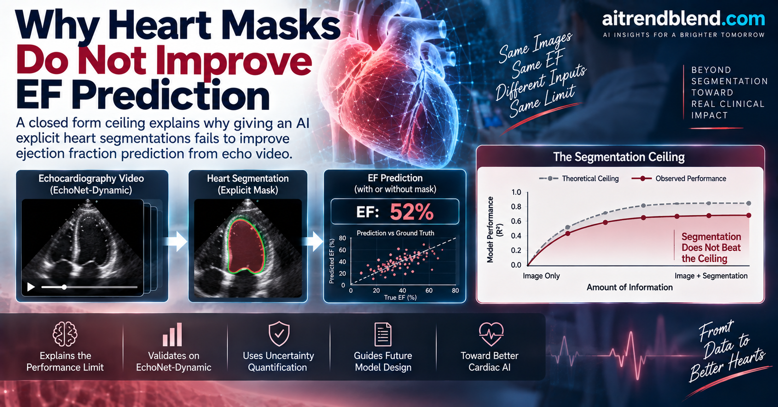
- The paper tests a widely held belief that giving an AI explicit heart segmentations should improve its prediction of ejection fraction from echocardiography video, and finds that it does not.
- It derives a closed form criterion the authors call the segmentation ceiling, showing that because ejection fraction is a difference of two volumes, small tracing errors get amplified.
- A realistic segmenter would need to hold per frame area error below about 10.5 percent to help, but a strong representative one sits near 14 percent, above the ceiling.
- Four separate ways of feeding the model segmentation or area information all fail to beat a plain raw video model, and perfect masks only help by leaking the answer.
- With input representation ruled out, the real lever is generalization and calibrated uncertainty, and the authors offer a simple recipe for both.
The number a cardiologist cannot do without
Ejection fraction, usually shortened to EF, measures the share of blood that leaves the left ventricle during a contraction. A healthy heart ejects somewhere north of half its filled volume with each beat. When that fraction drops, it is often the first quantitative sign of heart failure or a weakening heart muscle, which is why EF shows up in risk assessments, treatment choices, and the long term monitoring of patients living with cardiovascular disease.
Measuring it by hand is laborious. A sonographer or cardiologist finds the two extreme moments of the heartbeat, the fully relaxed end diastole and the fully squeezed end systole, traces the inner boundary of the ventricle on each, estimates a volume from that outline, and applies a geometric formula. Every step invites disagreement. Two experts tracing the same murky ultrasound frame can land on noticeably different numbers, and the images themselves are full of speckle, shifting views, and the ordinary variability of scanning a moving organ inside a living person.
That difficulty is precisely why automation is attractive. The public EchoNet-Dynamic dataset from Stanford, with more than ten thousand labeled echocardiograms, opened the door to video models that read EF directly from the clip. A convolutional architecture called R(2+1)D became the standard strong baseline, and later transformer designs narrowed the gap to expert agreement. The field has been productive. But it carried an assumption forward that almost nobody had tested head on.
The intuition that seems obvious, and the study that tests it
Here is the belief in plain form. Because EF is defined through the traced volumes of the ventricle, a model that is handed those traces, or taught to produce them, should predict EF more accurately than one squinting at raw pixels. It feels almost self evident, and a large body of work has accordingly bolted segmentation onto EF estimation in one way or another.
The authors, Farshid Farhadi Khouzani and colleagues, asked whether that actually helps a strong end to end video regressor, as opposed to simply mimicking the classical hand calculation. Their answer, argued both on paper and in careful experiments, is that it does not, and the reason is not a failure of engineering. It is baked into the definition of the quantity itself. This is the kind of negative result that is more valuable than most positive ones, because it saves an entire subfield from chasing a dead end, and it connects to a thread other groups have tugged at, including the observation in our coverage of HSS-Net and ejection fraction that a segmenter can score beautifully on overlap and still produce a poor EF.
Why subtracting two volumes is where the trouble starts
The heart of the argument is a short piece of algebra, and it rewards a slow read. Ejection fraction is a normalized difference.
Now imagine the segmenter does not measure those two volumes perfectly. It estimates each with some small relative error, a slight over or under estimate at end diastole and another at end systole. The question is how those two small errors flow into the final EF number. Working it through to first order, the authors arrive at a compact expression for how much error EF inherits.
Three things fall out of that one line, and each matters. The first is the multiplier at the front. Because EF subtracts two similar volumes, a given percentage error in the volumes gets scaled by how much blood remains in the ventricle, so the same tracing sloppiness bites harder in some hearts than others. The second is the correlation term. If the segmenter makes the same directional mistake at both moments, those errors partly cancel when you take the ratio, because a consistent scale factor divides out. If the two errors are independent, nothing cancels and the damage is maximal. The third, and the point of the whole exercise, is that this is quantitative. You can plug in numbers and get a hard threshold.
And the numbers are unforgiving. Under the worst case of independent errors, a segmenter would need to hold its per frame area error to around 7 percent just to match the regressor’s own accuracy of roughly 4.1 EF points. The authors then measured the real correlation between the two errors on the actual data and found it to be moderate, about 0.52, which relaxes the requirement. Even so, the break even sits at about 10.5 percent per frame area error. That is the ceiling. A mask that is any less accurate than that carries no net benefit for EF, no matter how you feed it in.
So how good is a realistic segmenter? The authors trained a standard DeepLabV3 network and measured it operating at about 13.8 percent area error, which lands it above the ceiling. In fact its induced EF error works out to roughly 5.4 EF points, larger than the regressor’s own error. The prediction is therefore blunt. A representative modern segmenter is not accurate enough to help, and might even hurt.
Four ways to feed the model a mask, four disappointments
A closed form argument is only as good as its evidence, so the team tested it four different ways, each compared against a raw video baseline that was architecturally identical except that its extra mask channel was set to zero. That control is important. It isolates the effect of the mask content itself rather than any change in the network’s shape.
The first strategy simply added the predicted segmentation as a fourth input channel alongside the three image channels. The second biased the clip sampling so that every training clip actually contained the crucial end diastole and end systole frames, on the theory that showing the model the volumetric extremes might help. The third added an auxiliary task that asked the model to predict the ventricular area at each moment in the clip. The fourth went further and derived a second EF estimate directly from that predicted area trajectory, using smooth differentiable maximum and minimum operators, then forced it to agree with the true EF.
None of them beat the plain baseline. The table below tells the story cleanly.
| Configuration | Val R squared | Test R squared | MAE | Val to test gap |
|---|---|---|---|---|
| Zero mask baseline (raw video) | 0.819 | 0.803 | 4.11 | 0.016 |
| Plus predicted mask channel | 0.790 | 0.766 | 4.46 | 0.024 |
| Plus end diastole and systole sampling | 0.799 | 0.773 | 4.49 | 0.026 |
| Plus per bin area consistency | 0.818 | 0.791 | 4.23 | 0.027 |
| Plus amplitude consistency | 0.830 | 0.792 | 4.24 | 0.038 |
Every segmentation or area guided strategy lands below the raw video baseline, and each one widens the gap between validation and test performance.
The amplitude experiment is the most revealing, because it separates mechanism from benefit. The auxiliary head genuinely learned a volume trajectory whose swing tracked true EF during training. The mechanism worked. Yet it produced no accuracy gain, and it actually widened the gap between validation and test, meaning the extra machinery fit the validation patients without transferring to new ones. Forcing the model to build an explicit internal picture of ventricular volume added nothing beyond what the regression head already pulls from the raw pixels. The available EF signal is bounded, and a strong video model already presses right up against that bound.
The trap of the perfect mask
There is one setting where masks appear to help enormously, and it is a cautionary tale worth telling on its own. When the authors fed in the ground truth expert tracings as the extra channel, test performance leapt to an R squared of about 0.97, far above anything else. That looks like a triumph until you remember where the EF labels come from. They are computed from those very same expert tracings. Handing the model the ground truth mask is quietly handing it the answer key. The authors flag this plainly as label leakage and report it only as an upper reference, never as a deployable result.
This is a subtle failure mode that can trap anyone building segmentation guided pipelines, and it is why they verified that the predicted masks were otherwise perfectly reasonable. The predicted per frame areas correlated with the truth at about 0.96, a genuinely good segmenter by ordinary standards. The residual error of roughly 14 percent is small in absolute terms, yet it is enough to poison the EF estimate once it passes through that amplifying difference of volumes. The limitation is not bad localization. It is arithmetic.
The mask is not too blurry or too crude. It is a good mask. The trouble is that ejection fraction subtracts two nearly equal volumes, and that subtraction magnifies whatever small error the mask carries.A plain reading of the segmentation ceiling
If the input is not the bottleneck, what is?
Having ruled out the input representation, the authors turned to the question that actually moves the needle. If a better mask will not help, what will? Their answer is generalization, the gap between how a model does on data it trained near and data it has never seen.
Their recipe is refreshingly plain. Keep an exponential moving average of the model weights during training, a technique that smooths out the noisy final weights into a more robust version, and pair it with strong but sensible video augmentation. The augmentations respect the physics of the problem. Horizontal flips are fine because area does not change under reflection, and gentle intensity and rotation changes mimic the variation across ultrasound machines and probe angles. This combination did not raise the accuracy ceiling, but it dramatically tightened the generalization gap, shrinking the difference between validation and test performance from 0.016 down to 0.009, the smallest of any configuration and close to the convolutional baseline’s own gap.
| Model, matched dense evaluation | Val R squared | Test R squared | MAE | RMSE |
|---|---|---|---|---|
| R(2+1)D convolutional baseline | 0.817 | 0.811 | 4.01 | 5.32 |
| UniFormer-S with weight averaging | 0.819 | 0.803 | 4.11 | 5.43 |
| UniFormer-S with averaging and augmentation | 0.815 | 0.806 | 4.08 | 5.39 |
The modern transformer matches the convolutional baseline once evaluation is made strictly comparable. All the confidence intervals overlap, so no model is meaningfully ahead.
A methodological point sits underneath this table that deserves applause. The authors noticed that different papers average their predictions over different numbers of video clips, and that this alone can shift the reported score enough to fake an improvement. They insisted on a matched dense protocol where every model averages over the same clips, then reported that their transformer and the older convolutional baseline are statistically indistinguishable. They explicitly decline to claim a new best result. In a field crowded with fractional gains that evaporate under scrutiny, that honesty is the point, not a footnote.
Knowing when the model does not know
A single EF number is not much use to a clinician without a sense of how much to trust it, so the paper closes with uncertainty. The common quick fix is to leave dropout switched on at prediction time and run the model many times, treating the spread of answers as a confidence estimate. The authors tried this and found it nearly useless here. The spread barely correlated with the model’s actual error, and the intervals it produced were badly overconfident. The perturbations from dropout produced a roughly constant uncertainty that told you almost nothing about which predictions to doubt.
Their alternative is to train the network to report its own uncertainty directly, predicting both an EF value and a variance for each video, using a formulation known as beta-NLL that is designed to keep the accuracy of the prediction intact while learning a meaningful spread.
This costs a little accuracy, dropping the R squared to about 0.755, but it buys uncertainty that actually means something. The predicted spread correlated with the real error, and after a single scaling factor fit on the validation set, the confidence intervals reached about 93 percent coverage, close to their nominal target. Most tellingly, the model reported larger uncertainty on lower EF cases, which are both rarer in the data and harder to assess clinically. In other words it expressed the most doubt exactly where a weakened heart makes the reading trickiest. That is the behavior you want from a tool meant to flag its own shaky answers, and it echoes a theme in our look at why models are confident when they should not be.
The clinical translation gap
It is worth drawing a careful line between what this paper demonstrates and what a hospital would need. An R squared around 0.81 and a mean error near 4 EF points is a respectable research result on a benchmark, but EF decisions in care hinge on thresholds and trends in individual patients, not on an average fit across a curated dataset. The paper does report strong performance at the clinically meaningful cutoffs, with the model discriminating reduced function well across the standard EF thresholds, and that threshold behavior generalized more cleanly than the continuous number did. That is encouraging, and it is the sort of result that matters clinically more than a raw correlation.
Even so, none of this makes the system ready to guide treatment. It was trained and tested on one institution’s data from a single stretch of years, using a single ultrasound view, and it has not been validated prospectively or across hospitals. The value of the work for a clinician is not a deployable EF engine. It is a clear eyed map of where effort should and should not go, plus a calibrated reliability signal that could one day accompany an automated reading. The distance between a benchmark and a bedside tool is measured in external validation, regulatory review, and the slow accumulation of evidence that the model behaves on scanners and patients it never trained on. This work sits firmly on the research side of that gap, and reads as a study rather than a product.
Honest limitations, including the clinical ones
The authors are unusually forthright about the boundaries of their claims, and several deserve emphasis. Everything rests on the EchoNet-Dynamic dataset, which comes from a single hospital over a single window of years. The cohort shift the authors observed even within that one dataset is itself a warning that behavior on data from another institution or another scanner is unknown. External validation is not a nicety here, it is the essential next step.
The analysis also uses a single apical four chamber view, while clinical EF is often estimated from two views combined, so a single view ceiling might differ from a two view one. The ceiling derivation is a first order approximation summarized at a representative EF and error scale, and although the authors measured the crucial error correlation directly rather than assuming it, the formula still reduces a patient by patient quantity to representative values, and it works on areas where true EF is defined on volumes, a simplification the authors note is conservative. The conclusions concern a segmenter near 14 percent area error, and the honest caveat is that a substantially more accurate segmenter, one that actually crosses the break even, could in principle help. None exists in that regime today, but the door is not bolted shut. Finally, the uncertainty estimates come from a single clip and a single model, their correlation with error is modest rather than strong, and the calibrated variant trades away a little accuracy for its honesty about doubt.
None of these caveats weakens the central contribution. They sharpen it. The paper does not claim a universal law, it claims a concrete, testable criterion together with the evidence that today’s segmenters fall on the wrong side of it, and it says exactly what would change that verdict. For readers tracking how the field wrestles with the disconnect between segmentation quality and clinical usefulness, our coverage of RABR-Net refining the boundaries that Dice scores miss and of a temporal attention module for cardiac segmentation are useful neighbors.
The core method, in runnable PyTorch
The block below is a faithful, self contained reference implementation of the paper’s key pieces, namely the closed form segmentation ceiling calculator, a four channel mask guided regressor around a compact video backbone stand in, the exponential moving average of weights, the differentiable amplitude consistency estimate, and the heteroscedastic beta-NLL uncertainty head and loss, with a smoke test. It follows the analysis described in the paper. The authors released their own code, linked below, so treat this as a compact teaching version rather than their exact implementation.
# The segmentation ceiling for ejection-fraction regression.
# Closed-form criterion, a mask-guided video regressor, EMA weights,
# the amplitude-consistency estimate, and a beta-NLL uncertainty head.
import copy, math
import torch
import torch.nn as nn
import torch.nn.functional as F

# ----------------------------------------------------------------------
# 1. The segmentation ceiling (Eq. 4): induced EF error from area error
# ----------------------------------------------------------------------
def induced_ef_error(area_err, ef=0.60, rho=0.52):
    """Std of EF error (in EF fraction) given per-frame relative area error.
    area_err and the return value are fractions, so multiply by 100 for EF points."""
    return (1.0 - ef) * area_err * math.sqrt(2.0 * (1.0 - rho))

def break_even_area_error(model_mae_ef_points, ef=0.60, rho=0.52):
    """Largest per-frame area error (percent) at which a mask can still help."""
    sigma_ef = model_mae_ef_points / 100.0                 # EF points -> fraction
    area_err = sigma_ef / ((1.0 - ef) * math.sqrt(2.0 * (1.0 - rho)))
    return 100.0 * area_err

# ----------------------------------------------------------------------
# 2. Mask-guided video regressor (compact backbone stand-in for UniFormer)
# ----------------------------------------------------------------------
class VideoBackbone(nn.Module):
    """Lightweight 3D conv stand-in. Swap for UniFormer-S in practice."""
    def __init__(self, in_ch=4, width=64):
        super().__init__()
        self.net = nn.Sequential(
            nn.Conv3d(in_ch, 32, 3, stride=(1, 2, 2), padding=1), nn.GroupNorm(8, 32), nn.SiLU(),
            nn.Conv3d(32, width, 3, stride=2, padding=1), nn.GroupNorm(8, width), nn.SiLU(),
            nn.Conv3d(width, width, 3, stride=(1, 2, 2), padding=1), nn.GroupNorm(8, width), nn.SiLU())
        self.width = width

    def forward(self, x):
        # x: (B, C, T, H, W) -> features (B, width, T')
        f = self.net(x)
        return f.mean(dim=(3, 4))                          # spatial pool -> (B, width, T')

class EFRegressor(nn.Module):
    def __init__(self, width=64, heteroscedastic=True):
        super().__init__()
        self.backbone = VideoBackbone(in_ch=4, width=width)
        self.drop = nn.Dropout(0.5)
        self.het = heteroscedastic
        self.head = nn.Linear(width, 2 if heteroscedastic else 1)
        self.area_head = nn.Linear(width, 1)              # per-bin LV area (auxiliary)
        nn.init.constant_(self.head.bias[0:1], 0.55)    # bias to dataset-mean EF

    def forward(self, clip):
        # clip: (B, 4, T, H, W); channel 4 is the mask (zeros = raw-video baseline)
        feat_t = self.backbone(clip)                     # (B, width, T')
        area = self.area_head(feat_t.transpose(1, 2)).squeeze(-1)  # (B, T') area sequence
        pooled = self.drop(feat_t.mean(dim=2))            # (B, width)
        out = self.head(pooled)
        if self.het:
            mu, logvar = out[:, 0], out[:, 1].clamp(-6, 3)
            return mu, logvar, area
        return out[:, 0], None, area

# ----------------------------------------------------------------------
# 3. Differentiable amplitude-consistency EF from the area sequence (Eq. 6)
# ----------------------------------------------------------------------
def amplitude_ef(area, beta=8.0, eps=1e-4):
    soft_max = (F.softmax(beta * area, dim=1) * area).sum(1)   # soft maximum
    soft_min = (F.softmax(-beta * area, dim=1) * area).sum(1)  # soft minimum
    return (soft_max - soft_min) / (soft_max + eps)         # EF-like amplitude ratio

# ----------------------------------------------------------------------
# 4. beta-NLL heteroscedastic loss (Eq. 10), beta = 0.5
# ----------------------------------------------------------------------
def beta_nll(mu, logvar, y, beta=0.5):
    var = torch.exp(logvar)
    nll = 0.5 * ((y - mu) ** 2 / var + logvar)
    weight = var.detach() ** beta                        # stop-gradient reweighting
    return (weight * nll).mean()

# ----------------------------------------------------------------------
# 5. Exponential moving average of weights (decay 0.999)
# ----------------------------------------------------------------------
class EMA:
    def __init__(self, model, decay=0.999):
        self.decay = decay
        self.shadow = copy.deepcopy(model).eval()
        for p in self.shadow.parameters(): p.requires_grad_(False)

    @torch.no_grad()
    def update(self, model):
        for s, p in zip(self.shadow.parameters(), model.parameters()):
            s.mul_(self.decay).add_(p, alpha=1.0 - self.decay)

# ----------------------------------------------------------------------
# 6. Smoke test on dummy data
# ----------------------------------------------------------------------
if __name__ == "__main__":
    # the ceiling in numbers: break-even vs a 13.8% segmenter
    be = break_even_area_error(model_mae_ef_points=4.1, ef=0.60, rho=0.52)
    seg = induced_ef_error(0.138, ef=0.60, rho=0.52) * 100
    print(f"break-even area error: {be:.1f}%")          # about 10.5%
    print(f"13.8% segmenter induces: {seg:.1f} EF points") # about 5.4

    B, T, H, W = 2, 16, 64, 64
    model = EFRegressor(heteroscedastic=True)
    ema = EMA(model)
    clip = torch.randn(B, 4, T, H, W); clip[:, 3] = 0   # zero-mask = raw-video baseline
    y = torch.tensor([0.58, 0.32])
    mu, logvar, area = model(clip)
    loss = beta_nll(mu, logvar, y) + 0.1 * F.mse_loss(amplitude_ef(area), y)
    loss.backward(); ema.update(model)
    print("pred EF:", mu.detach().tolist(), "| loss:", float(loss), "| ok")
Conclusion
The central contribution of this work is a piece of clarity that the field needed. A widely pursued idea, that explicit heart segmentation should sharpen automated ejection fraction, turns out to be wrong for a reason that is not accidental but structural. Because EF is a normalized difference of two similar volumes, any error in tracing those volumes gets amplified, and the authors made that amplification precise enough to yield a hard accuracy threshold. Below roughly 10 percent per frame area error a mask can help, above it a mask hurts, and today’s segmenters live on the wrong side of that line.
What elevates the paper is that it did not stop at the equation. It confirmed the prediction four different ways, watched even a mechanically successful auxiliary task fail to transfer, and caught the seductive trap of the ground truth mask that appears to work only because it leaks the answer. That combination of a closed form argument and controlled experiments is how a negative result earns real authority, and it is far more useful than yet another architecture claiming a fractional gain.
The honesty of the evaluation is its own contribution. By insisting that every model average over the same clips, the authors showed that a modern transformer and an older convolutional baseline are statistically tied, and they declined to dress that up as an improvement. The lesson they draw, that the real lever is generalization and calibrated uncertainty rather than input representation, points the field toward larger and more diverse data and toward models that report their own doubt, which is a more productive place to spend effort than better preprocessing.
The limitations are real and clearly stated. A single institution, a single view, a first order approximation, and an uncertainty signal that is informative rather than sharp. The clinical translation gap remains wide, and nothing here is ready to guide a treatment decision. But the ceiling itself is portable. It is a design criterion any team can apply by measuring their own segmenter, and it says precisely when investing in better segmentation would pay off and when it would be wasted.
Read as a new leaderboard entry, this paper deliberately is not one. Read as an explanation, which is why a natural and heavily pursued direction saturates and what to do instead, it is a small and valuable correction to the collective intuition of a whole subfield. In medical AI, where a misplaced belief can send years of effort in the wrong direction, a clean account of what does not work, and why, is worth as much as most accounts of what does.
Frequently asked questions
What is the segmentation ceiling in plain terms?
It is a formula that says how accurate a heart segmentation must be before it can improve an AI’s ejection fraction prediction. Because ejection fraction is a difference of two volumes, small tracing errors get amplified, so a mask must hold its per frame area error below about 10.5 percent to help. Realistic segmenters sit above that line.
Why does adding a segmentation mask make the prediction worse?
A realistic mask carries roughly 14 percent area error. When that error passes through the difference of two similar volumes that defines ejection fraction, it is magnified into an error larger than the raw video model’s own. The mask injects a misleading area signal rather than useful structure, so accuracy drops slightly.
Why did the perfect mask score so well?
Feeding the ground truth expert tracing produced an artificially high result because the ejection fraction labels are themselves computed from those same tracings. The model was effectively handed the answer, a case of label leakage, so the authors report it only as an upper reference and never as a usable configuration.
If masks do not help, what does?
Generalization. Keeping an exponential moving average of the model weights and applying strong but physically sensible augmentation tightened the gap between validation and test performance without sacrificing accuracy. The authors argue that larger and more diverse data, not better preprocessing, is where future gains will come from.
How does the uncertainty part work?
Rather than leaving dropout on at inference, which gave uninformative uncertainty here, the model is trained to predict both an ejection fraction and its variance directly. After a single calibration step this produced well calibrated intervals and, usefully, larger uncertainty on the harder low ejection fraction cases.
Is this ready for clinical use?
No. It is a research preprint trained and tested on one institution’s data with a single ultrasound view, and it has not been peer reviewed, validated across hospitals, or cleared for clinical use. Its value is a design criterion and a calibrated reliability signal, not a deployable ejection fraction tool.
Read the source research
This analysis is based on the preprint by Farshid Farhadi Khouzani, Paul La Plante, Bryar Mustafa Shareef, and Laxmi Gewali. The authors released their code publicly.
Citation. Farhadi Khouzani, F., La Plante, P., Shareef, B. M., and Gewali, L. The segmentation ceiling, why explicit left-ventricular masks do not improve learned ejection-fraction regression. arXiv preprint arXiv:2609.19730 (2026). Experiments use the publicly available EchoNet-Dynamic dataset under a Stanford Research Use Agreement. This analysis is based on the published paper and an independent evaluation of its claims, and is not medical advice.