
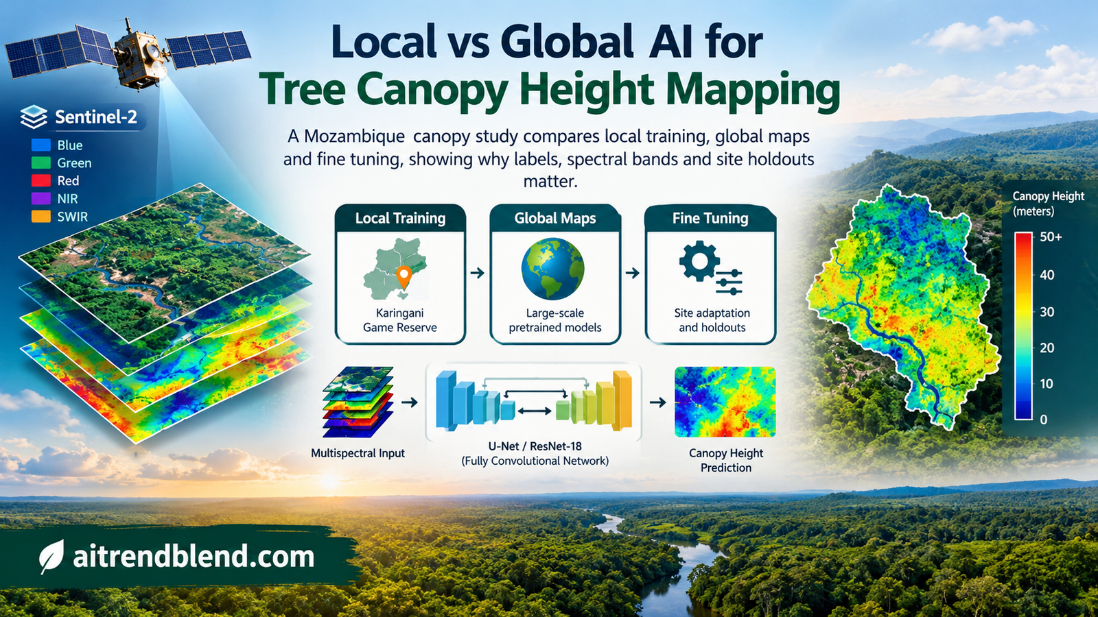
A reserve manager opens a global tree height map to inspect vegetation around a river. The image looks detailed, and the model behind it has performed well across the world. Yet the immediate question is local. Does it distinguish the shorter canopy, scattered trees and ecological variation inside this reserve well enough to support the analysis? A new comparison from Mozambique shows why that answer cannot be read from a global benchmark.
- A small fully convolutional network trained with local labels achieved the lowest canopy height error among the methods tested in Karingani Game Reserve.
- The local FCN reached an average RMSE of 1.64 metres compared with 2.43 metres for the strongest evaluated global map.
- Global pretraining helped some comparisons but did not produce the best local model in this study.
- Site sampling, spectral bands and architecture changed error by similar amounts in the controlled comparisons.
- Height accuracy and a calibrated biomass proxy gave different rankings, so the evaluation target matters.
- The evidence comes from one reserve and one prediction task. It does not show that local models generally replace global mapping.
Local usefulness is a separate modeling objective
Esther Rolf of the University of Colorado Boulder and Lucia Gordon, Milind Tambe and Andrew Davies of Harvard University investigate this question in their JMLR study contrasting local and global satellite modeling. The task is tree canopy height estimation in Karingani Game Reserve, a roughly 145,000 hectare landscape in Mozambique near the South African border. Its savanna vegetation varies across geology, terrain, rainfall and proximity to rivers.
The study compares three routes to a usable local map. A team can crop an existing global product, adapt a model that has already seen global data, or train a new model using local labels. These choices involve different resources. A published map is available without a new training run. Local training requires imagery, reference measurements and evaluation. Fine tuning requires compatible inputs and accessible model weights as well as local labels.
The contribution is a comparison of those routes and the decisions around them. The authors do not introduce a new foundation model. Their best result comes from a modest convolutional network. What makes the study useful is the way it tests whether global progress translates into local accuracy, then asks which parts of the workflow account for the remaining differences.
This belongs in the broader Machine Learning category. Its central lesson concerns distribution, supervision and evaluation design. A model can resolve variation between widely separated ecosystems while struggling to resolve the smaller variation that matters inside one ecosystem. Both results can be true without either evaluation being wrong.
The reference labels change what can be learned
The local reference data cover 24 sites surveyed in May and early June 2021. A drone carried the Harvard Animal Landscape Observatory sensor system, including LiDAR, navigation and positioning equipment. The resulting canopy height maps have a spatial resolution of one metre. The authors report that collecting data took roughly one day per site, including travel.
These are valuable labels, even if the resulting neural network is small. The study reports processed LiDAR horizontal accuracy below one centimetre and vertical accuracy below two centimetres. Those positioning and processing figures should not be confused with a direct error bound on every derived canopy height label. Converting a point cloud into a canopy surface introduces its own modeling choices.
The satellite inputs for the local experiments come from three Sentinel-2 tiles acquired on 13 May 2021, near the LiDAR survey period and with low cloud cover across the sites. The main model uses twelve spectral bands aligned to a ten metre grid. Local labels cover only part of the reserve, so the practical task is to extend predictions into areas without drone reference coverage.
The label definition is easy to overlook. Heights above 30 metres are treated as missing and negative heights become zero. The authors report that 99.95 percent of valid original height pixels already fall within that range. When coarsening the reference raster from one metre to ten metres, they use the 90th percentile of the contributing heights. A prediction therefore targets this aggregated height statistic, rather than the mean of all vegetation inside the cell.
This formulation expresses the preprocessing described in the paper. It is not a newly proposed loss. Replacing that percentile with a mean would change the regression target and make a claimed reproduction difficult to interpret. Alignment, missing values and aggregation belong in the model specification because they decide what a correct output means.
The paper also distinguishes the local labels from GEDI measurements used in earlier global mapping efforts. Global coverage is a major advantage of GEDI, but sampling and geolocation error have different implications from dense local drone measurements. The observed benefit of local training therefore combines regional relevance with a different supervision source. It is not an experiment that changes geography while holding label quality constant.
A spatial split asks the deployment question
The authors divide the 24 sites into twelve training sites, six validation sites and six test sites. They construct four such spatial splits so that every site appears once in testing and once in validation. Test sites are excluded from both parameter fitting and hyperparameter selection. This resembles using surveyed areas to predict other areas of the same reserve.
Why not randomly divide the pixels? Nearby pixels share vegetation, illumination, geology and spatial texture. Placing adjacent portions of the same site in training and testing can reward a model for recognizing local context it has effectively already encountered. Holding out whole sites asks a harder and more relevant question about geographic extension.
The four splits still concern the same reserve. They do not establish transfer to another country, a different biome or a later disturbance season. They also contain spatially related observations, so millions of evaluated pixels should not be interpreted as millions of independent landscapes. The unit of deployment and the unit of uncertainty need to remain visible.
Choose the holdout unit before choosing the architecture. If the intended use is prediction at unsurveyed sites, evaluate at unsurveyed sites. Report which sites contributed to model selection and retain a separate account of how error varies among landscapes.
The study selects hyperparameters and checkpoints using validation mean squared error, with training limited to 200 epochs. Neural models use AdamW and a scheduler that reduces the learning rate after validation performance plateaus. Initial learning rate and weight decay are each searched over four values from \(10^{-5}\) to \(10^{-2}\). The test data are reserved for reporting performance after those choices.
The small network has enough context for this task
The best local model is a fully convolutional network with five feature layers and 128 filters per layer. Its twelve channel version has 604,417 parameters and an eleven by eleven pixel receptive field. It outputs a dense height map. There is no classification head, no canopy category threshold and no requirement to identify individual tree instances.
Five consecutive convolutions with three by three kernels expand the receptive field to eleven pixels when stride remains one and no pooling is used. A final one by one convolution maps the feature channels into one height value. The implementation below follows this architecture, with leaky rectified activations and a linear regression output.
The training objective is ordinary pixelwise mean squared error. When reference pixels are missing, the editorial implementation evaluates that objective only on valid pixels. It leaves predictions unconstrained rather than applying a sigmoid or clipping them before calculating error. Those additions would change the regression behavior and should be evaluated as separate decisions.
Other models provide useful context. XceptionS2 uses residual convolutional blocks. A U-Net with a ResNet-18 backbone uses a larger image context. A pixelwise random forest sees the spectral features of one pixel without spatial texture. These comparisons let the authors separate some benefits of local calibration from the value of learning surrounding image structure.
The result does not identify a universal optimum in model size. The random forest is simpler but performs worse than the FCN. The larger networks also perform worse in the reported setup. A reasonable interpretation is that this target, label set and spatial extent benefited from a particular amount of context and capacity. The neighboring article on pruning and generalization explores a different route to understanding capacity, rather than supplying proof for the ecological result here.
What the height comparisons actually show
Table 1 provides the clearest common reference for the reported metrics. The values below use that table rather than mixing rounded values from different figures. Performance is evaluated at ten metre resolution unless otherwise stated, with the reported averages combining the four spatial splits. The table also reports standard deviations from ten training runs, which should not be treated as confidence intervals for performance across all African savannas.
| Model or map | Training route | RMSE in metres | MAE in metres | Height R squared |
|---|---|---|---|---|
| Local FCN | Local labels and random initialization | 1.64 | 1.20 | 0.57 |
| XceptionS2 without location layers | Local labels and random initialization | 1.94 | 1.47 | 0.40 |
| XceptionS2 with global initialization | Global supervision then local adaptation | 1.98 | 1.48 | 0.37 |
| U-Net with pretrained encoder | Global self supervision then decoder adaptation | 2.05 | 1.54 | 0.32 |
| U-Net with random initialization | All model parameters trained locally | 2.27 | 1.59 | 0.10 |
| Pixelwise random forest | Local labels without spatial context | 2.28 | 1.80 | 0.16 |
| GLAD from Potapov and colleagues | Existing global map | 3.09 | 2.44 | \(-0.53\) |
| ETH from Lang and colleagues | Existing global map | 4.51 | 3.83 | \(-2.26\) |
| Meta from Tolan and colleagues | Existing global map | 3.51 | 2.87 | \(-0.98\) |
| Pauls and colleagues | Existing global map | 2.43 | 2.01 | 0.05 |
The FCN improves average RMSE by 0.79 metres relative to the best evaluated global map, a reduction of about 33 percent as reported by the authors. Its improvement over the best globally initialized and locally adapted model is 0.34 metres, about 17 percent. These are comparisons within the study, with its chosen models, labels and evaluation grids.
The negative height R squared values for several maps are also informative. Under the reported calculation, those predictions perform worse in squared error than the corresponding constant mean reference. Negative R squared does not mean negative correlation by definition. Bias in the predicted level can produce a poor squared error comparison even when a map contains some useful relative structure.
That distinction helps explain why a global product can still have value while losing this local comparison. The paper notes that the evaluated global maps have lower RMSE in Karingani than in their broader global evaluations. The reserve is therefore not simply an unusually disastrous location for them. Yet locally trained alternatives still improve substantially on those local errors.
Higher spatial resolution does not settle the ranking either. The original GLAD product is coarser than the Meta product, but GLAD has lower height RMSE in this evaluation. Fine texture can make a map look more convincing without making its numerical canopy height values more accurate. Resampling to a common evaluation grid also does not make the original inputs, label definitions or acquisition dates identical.
Pretraining helps a route without winning the comparison
The local adaptation experiments use two types of pretraining. XceptionS2 starts from supervised global canopy height weights, specifically model zero from the published ensemble. The U-Net uses an encoder pretrained through SSL4EO on global satellite imagery. These are distinct transfer settings, so a result from one should not be treated as a test of every possible geospatial foundation model.
A detail in the Table 1 caption deserves attention. Only the last three layers are tuned for all three XceptionS2 variants, including those initialized randomly. This is a comparison of the stated adaptation procedures. It is not a clean demonstration that full optimization from random initialization always matches or beats full optimization of a pretrained network.
The U-Net comparison tests both decoder adaptation and adaptation of the entire pretrained model. The former reaches an average RMSE of 2.05 metres, while adapting everything reaches 2.08 metres. The randomly initialized version reaches 2.27 metres and has substantially greater reported variability. Pretraining can therefore help within an architecture even while the best overall local solution comes from a different architecture.
Coverage of the global alternatives is also incomplete for practical reasons. Fine tuning the Meta model would have required purchasing proprietary imagery, and weights for the Pauls model were not publicly available when the experiments were conducted. Those are historical constraints of this study, rather than claims about what is available today. The paper evaluates their maps but does not test those two models under the same local adaptation procedure.
“global and local mapping may constitute distinct modeling goals”Rolf, Gordon, Tambe and Davies, conclusion of the published study.
Data decisions compete with architecture decisions
The controlled experiments make the paper more useful than a single ranking table. The authors vary model architecture, input bands and the number of training sites. Relative to the main FCN configuration, changing from FCN to the next best local model changes average RMSE by 0.30 metres. Using RGB instead of all twelve input channels changes it by 0.22 metres. Using three training sites instead of twelve changes it by 0.25 metres.
Those comparisons do not prove equal returns for every possible investment. They show that the tested data decisions can move error by amounts comparable to the tested architecture decision. A team that spends all of its effort replacing the backbone while ignoring where labels come from could miss an equally consequential part of the workflow.
Adding a near infrared channel to RGB reduces average FCN RMSE by about ten percent in the reported experiment. The remaining eight bands provide a smaller additional improvement. Location embeddings do not improve the best local configuration appreciably and can slightly worsen it. A geographic coordinate can be useful for interpolation while becoming less helpful when the evaluation asks for extension to unseen sites.
Spatial context and input coverage are different issues. The site’s analysis of multiple remote sensing sources offers a neighboring example of feature design. Here, however, the experiment changes spectral channels within the stated satellite input setup. It does not establish that adding another sensor would yield the same improvement.
The training subset experiment also shows substantial variability. With fewer sites, performance usually worsens on average and varies more between subsets. Some smaller subsets produce strong individual runs. That is not a recommendation to discard data. The authors explain that their experiment cannot fully separate favorable site composition from favorable random model initialization.
Benchmark the data plan alongside the model plan. Compare spectral inputs and site coverage using the same held out sites. Keep the amount of training exposure controlled when changing the number of sites, and examine variability instead of selecting the most flattering subset.
A biomass proxy asks a different question
Canopy height maps are often used as ingredients in ecological calculations. The study therefore asks whether the maps preserve information useful for estimating relative aboveground biomass across sites. It first derives reference biomass estimates from the local LiDAR height labels using an established allometric relationship from Colgan and colleagues, cited in the paper.
These reference values are not direct measurements of harvested biomass. The study constructs a predictor using canopy cover and height, with canopy cover defined by height above 1.5 metres. It then fits an affine regression between each map’s site level predictor and the reference estimates across the 24 sites. The resulting goodness of fit measures the retained relative signal after this local calibration.
| Map | Reported R squared |
|---|---|
| Local FCN | 0.52 |
| Meta | 0.52 |
| Pauls and colleagues | 0.41 |
| GLAD | 0.22 |
| ETH | 0.11 |
Meta matches the local FCN on this fitted relationship despite having worse pixel height RMSE. For this biomass analysis, the Meta product is used at one metre resolution while the other map predictors use ten metre resolution. The target, aggregation and calibration have changed, so this table should not be merged with the pixel height leaderboard.
The fits use the 24 study sites and are not a separate prospective test of biomass prediction. They do not validate carbon accounting, carbon credits or reserve management decisions. Their value is narrower and useful. A map with biased absolute heights may retain some relative site structure after calibration, while a map with better pixel error need not dominate every ecological summary.
What to check before carrying the result elsewhere
The most consequential limitation is geographic scope. One reserve provides a controlled and detailed case study, not a representative sample of the planet’s vegetation. Tropical forest, dense urban trees and other savannas may demand different spatial context, labels and input imagery. The authors themselves expect their local models to perform poorly if applied globally without adaptation.
The global map comparison combines different source sensors, years, training labels, resolutions and objectives. Some error may arise from these mismatches rather than from training extent alone. The study establishes a practical local performance gap among the available routes. It does not experimentally identify a single cause of every gap.
The imagery was selected near the survey period with low cloud cover. Seasonal shifts, fire, drought and missing optical observations could change the problem. Our article on cloud affected optical imagery concerns a different method, but it illustrates why image availability belongs in an operational evaluation rather than being assumed away.
The network comparisons depend on the training protocol. The U-Net models exhibited problems near patch edges, and the authors used only the central four by four pixels of each 64 by 64 window when tiling those predictions to reduce that effect. Other optimization schedules, adaptation policies or boundary handling could change the rankings. No comparison covers every reasonable configuration.
The source normalizes locally trained model inputs using channel statistics across the three imagery tiles, including geography outside the labeled training sites. This uses unlabeled imagery from the study extent. The reference code instead fits normalization on training sites only and identifies that difference explicitly. Neither convention should be silently swapped when reproducing results.
Finally, this is height regression. The site’s satellite change detection analysis involves a different target and evidence standard. Terms such as local and global can also describe receptive fields inside a network, whereas this paper primarily contrasts the geographic extent of training and use. Keeping those meanings separate avoids a misleading comparison.
Build for the geography where the answer will be used
The paper’s achievement is a carefully grounded comparison of local mapping options. A small FCN trained on high quality local labels outperformed the evaluated global products and adapted models for canopy height in Karingani. The result makes local supervision a serious baseline rather than an afterthought to the largest available pretrained model.
The conceptual shift is from asking which model is best in aggregate to asking which learning and evaluation setup matches a particular region. Global products retain enormous value because they cover places without local surveys. Their global usefulness and their local adequacy should each be measured, rather than assumed to rise together.
The finding transfers as an experimental habit. Define the desired variable, align the grids, preserve the label statistic, hold out the relevant spatial unit and compare local training with local adaptation. Then vary the data choices as deliberately as the model choices. These steps are applicable beyond canopy height even when the eventual model ranking changes.
The limits remain visible. This reserve does not establish a universal preference for small networks, local labels are costly to collect, and the transfer experiments leave several possible adaptation routes untested. The biomass proxy also demonstrates that a ranking on one metric cannot substitute for evaluation of the intended downstream analysis.
A stronger next study would repeat the same comparison across different biomes, seasons and annotation budgets while testing adaptation methods designed for regional use. The immediate lesson is already practical. A global model supplies a starting resource. Local evidence decides whether it answers the question on the ground.
Complete PyTorch reference for the local FCN
The listing implements the complete local FCN with its custom spectral normalization and convolutional layers, masked squared error, site based splitting, training, hyperparameter selection, evaluation and a runnable synthetic smoke test. The default network matches the reported parameter count and receptive field. It is an editorial implementation, not a replacement for the authors’ full experimental repository.
The inputs are aligned spectral image tensors and canopy height tensors, with an optional helper for percentile aggregation of the fine resolution labels. Raster coordinate systems, cubic reprojection, raw imagery acquisition, pretrained alternatives and biomass calibration are outside this listing. The supplied fold structure must be populated with the actual sites for a real experiment. Artificial sites in the smoke test demonstrate the workflow only.
Training statistics use training sites only, and tiled prediction includes a five pixel context halo to prevent internal boundary seams for this FCN. Those are disclosed editorial choices. The smoke test trains a reduced width network for speed while separately checking the default architecture’s parameter count. No synthetic output is presented as the paper’s measured result.
Python syntax and independent numerical checks of aggregation, regression metrics and the architecture arithmetic passed. PyTorch is unavailable in this environment, so the included training smoke test has not been executed here. Run it after installing PyTorch before treating this reference as an executed implementation.
"""Editorial local FCN reference for Rolf et al., JMLR 27(45), 2026.

Requires Python 3.10+ and PyTorch. Run this file for a synthetic smoke test.
Aligned tensors are inputs, not raw GeoTIFFs: image [12,H,W], height [H,W].
Raster CRS checks, cubic reprojection, source imagery acquisition, pretrained
baselines and biomass calibration are outside this reference's scope.
The default FCN has 604,417 parameters and an 11x11 receptive field.
Training-only input statistics, deterministic crops, halo tiling and the dummy
site folds are editorial choices. They do not reproduce the published protocol.
"""
from copy import deepcopy
from dataclasses import dataclass
import math
import torch
from torch import nn
from torch.utils.data import Dataset, DataLoader


@dataclass
class Site:
    name: str
    image: torch.Tensor
    height: torch.Tensor


def coarsen_height(height_1m, factor=10):
    """Clean 1m labels, then aggregate each aligned block by its 90th percentile.

    This is block aggregation only. Align CRS, extent and grid externally.
    """
    values = torch.as_tensor(height_1m, dtype=torch.float32).clone()
    if values.ndim != 2 or factor < 1:
        raise ValueError("Expected a height raster and positive block factor.")
    h, w = values.shape
    if h % factor or w % factor:
        raise ValueError("Height dimensions must be divisible by block factor.")
    values[~torch.isfinite(values) | (values > 30)] = float("nan")
    values.clamp_(min=0)
    blocks = values.reshape(h // factor, factor, w // factor, factor)
    blocks = blocks.permute(0, 2, 1, 3).reshape(h // factor, w // factor, -1)
    return torch.nanquantile(blocks, .9, dim=-1)


def validate_sites(sites):
    if not sites or len({s.name for s in sites}) != len(sites):
        raise ValueError("Need nonempty sites with unique names.")
    channels = sites[0].image.shape[0]
    for site in sites:
        if site.image.ndim != 3 or site.height.ndim != 2:
            raise ValueError("Expected image [C,H,W] and height [H,W].")
        if site.image.shape[0] != channels or site.image.shape[1:] != site.height.shape:
            raise ValueError("All sites need consistent channels and aligned grids.")
        if not site.image.is_floating_point() or not site.height.is_floating_point():
            raise ValueError("Convert images and heights to floating point tensors.")


def split_sites(sites, groups, fold):
    """Four supplied groups of six sites give 12/6/6 train/validation/test.

    Each group is test once and validation once. Publication site assignments
    must be supplied for reproduction; the smoke test uses artificial groups.
    """
    validate_sites(sites)
    if len(groups) != 4 or any(len(group) != 6 for group in groups):
        raise ValueError("Need four groups with six site names each.")
    flattened = [name for group in groups for name in group]
    if len(set(flattened)) != 24 or set(flattened) != {s.name for s in sites}:
        raise ValueError("Groups must partition exactly the 24 supplied sites.")
    if not 0 <= fold < 4:
        raise ValueError("Fold index must be 0, 1, 2 or 3.")
    test_names = set(groups[fold])
    val_names = set(groups[(fold + 1) % 4])
    train = [s for s in sites if s.name not in test_names | val_names]
    val = [s for s in sites if s.name in val_names]
    test = [s for s in sites if s.name in test_names]
    assert not ({s.name for s in train} & (test_names | val_names))
    return train, val, test


class SpectralStandardizer(nn.Module):
    """Fit only on training sites, an explicit change from full-tile statistics."""
    def __init__(self, channels):
        super().__init__()
        self.register_buffer("mean", torch.zeros(1, channels, 1, 1))
        self.register_buffer("scale", torch.ones(1, channels, 1, 1))

    @torch.no_grad()
    def fit(self, sites):
        channels = self.mean.shape[1]
        total = torch.zeros(channels, dtype=torch.float64)
        squared = torch.zeros_like(total)
        count = torch.zeros_like(total)
        for site in sites:
            x = site.image.detach().cpu().double().reshape(channels, -1)
            valid = torch.isfinite(x)
            safe = torch.where(valid, x, 0)
            total += safe.sum(1)
            squared += safe.square().sum(1)
            count += valid.sum(1)
        if (count == 0).any():
            raise ValueError("Every band needs valid training observations.")
        mean = total / count
        variance = (squared / count - mean.square()).clamp_min(1e-12)
        self.mean.copy_(mean.float().reshape_as(self.mean))
        self.scale.copy_(variance.sqrt().float().reshape_as(self.scale))

    def forward(self, x):
        safe = torch.where(torch.isfinite(x), x, self.mean)
        return (safe - self.mean) / self.scale


class ConvFeatureLayer(nn.Module):
    def __init__(self, incoming, outgoing):
        super().__init__()
        self.convolution = nn.Conv2d(incoming, outgoing, 3, padding=1)
        self.activation = nn.LeakyReLU(negative_slope=.01)

    def forward(self, x):
        return self.activation(self.convolution(x))


class LocalCanopyFCN(nn.Module):
    def __init__(self, channels=12, width=128):
        super().__init__()
        self.normalize = SpectralStandardizer(channels)
        layers = [ConvFeatureLayer(channels, width)]
        layers += [ConvFeatureLayer(width, width) for _ in range(4)]
        self.features = nn.Sequential(*layers)
        self.height = nn.Conv2d(width, 1, kernel_size=1)

    def forward(self, image):
        # Linear regression head. No sigmoid, classification loss or clipping.
        return self.height(self.features(self.normalize(image)))[:, 0]


class SitePatches(Dataset):
    def __init__(self, sites, crop=64, samples_per_site=16, seed=0):
        validate_sites(sites)
        if min(min(s.height.shape) for s in sites) < crop:
            raise ValueError("Sites must be at least as large as the crop.")
        self.sites, self.crop = sites, crop
        self.samples_per_site, self.seed, self.epoch = samples_per_site, seed, 0

    def __len__(self):
        return len(self.sites) * self.samples_per_site

    def __getitem__(self, index):
        site = self.sites[index // self.samples_per_site]
        generator = torch.Generator().manual_seed(
            self.seed + 1000003 * self.epoch + index)
        h, w = site.height.shape
        row = int(torch.randint(h - self.crop + 1, (1,), generator=generator))
        col = int(torch.randint(w - self.crop + 1, (1,), generator=generator))
        x = site.image[:, row:row+self.crop, col:col+self.crop].float()
        y = site.height[row:row+self.crop, col:col+self.crop].float()
        valid = torch.isfinite(y) & torch.isfinite(x).all(dim=0)
        return x, y, valid


def masked_mse(prediction, target, valid):
    valid = valid & torch.isfinite(target)
    if not valid.any():
        return None
    if not torch.isfinite(prediction[valid]).all():
        raise FloatingPointError("Nonfinite prediction on valid target pixels.")
    return (prediction[valid] - target[valid]).square().mean()


@torch.no_grad()
def predict_tiled(model, image, tile=256):
    """Use a five-pixel context halo to avoid internal tile seams for this FCN."""
    model.eval()
    device = next(model.parameters()).device
    _, h, w = image.shape
    result = torch.empty((h, w), dtype=torch.float32)
    halo = 5
    for row in range(0, h, tile):
        for col in range(0, w, tile):
            end_row, end_col = min(row + tile, h), min(col + tile, w)
            top, left = max(0, row - halo), max(0, col - halo)
            bottom, right = min(h, end_row + halo), min(w, end_col + halo)
            patch = image[:, top:bottom, left:right].float().unsqueeze(0).to(device)
            prediction = model(patch)[0].cpu()
            result[row:end_row, col:end_col] = prediction[
                row-top:end_row-top, col-left:end_col-left]
    return result


@torch.no_grad()
def evaluate(model, sites):
    totals = torch.zeros(6, dtype=torch.float64)
    for site in sites:
        prediction = predict_tiled(model, site.image)
        valid = torch.isfinite(site.height) & torch.isfinite(site.image).all(0)
        target = site.height[valid].double()
        estimate = prediction[valid].double()
        if not torch.isfinite(estimate).all():
            raise FloatingPointError("Invalid model predictions.")
        error = estimate - target
        totals += torch.tensor([len(target), error.square().sum().item(),
                                error.abs().sum().item(), error.sum().item(),
                                target.sum().item(), target.square().sum().item()],
                               dtype=torch.float64)
    n, sse, absolute, signed, sy, sy2 = totals.tolist()
    if n == 0:
        raise ValueError("No valid evaluation pixels.")
    denominator = sy2 - sy * sy / n
    return {"n": int(n), "mse": sse/n, "rmse": math.sqrt(sse/n),
            "mae": absolute/n, "bias": signed/n,
            "r2": 1 - sse/denominator if denominator > 0 else float("nan")}


def fit_local(train, validation, lr=.001, weight_decay=.0001, epochs=200,
              crop=64, samples_per_site=16, width=128, seed=0):
    torch.manual_seed(seed)
    model = LocalCanopyFCN(train[0].image.shape[0], width)
    model.normalize.fit(train)
    patches = SitePatches(train, crop, samples_per_site, seed)
    loader = DataLoader(patches, batch_size=8, shuffle=True, num_workers=0,
                        generator=torch.Generator().manual_seed(seed))
    optimizer = torch.optim.AdamW(model.parameters(), lr=lr, weight_decay=weight_decay)
    scheduler = torch.optim.lr_scheduler.ReduceLROnPlateau(
        optimizer, mode="min", factor=.1, patience=10)
    best_loss, best_state = float("inf"), None
    history = []
    for epoch in range(epochs):
        patches.epoch = epoch
        model.train()
        updates = 0
        for x, y, valid in loader:
            optimizer.zero_grad(set_to_none=True)
            loss = masked_mse(model(x), y, valid)
            if loss is None:
                continue
            loss.backward()
            optimizer.step()
            updates += 1
        if not updates:
            raise ValueError("No valid training observations in this epoch.")
        metrics = evaluate(model, validation)
        scheduler.step(metrics["mse"])
        history.append(metrics)
        if metrics["mse"] < best_loss:
            best_loss = metrics["mse"]
            best_state = deepcopy(model.state_dict())
    if best_state is None:
        raise RuntimeError("No validation checkpoint selected.")
    model.load_state_dict(best_state)
    return model, history


def run_fold(sites, groups, fold=0, settings=None, **training_options):
    train, validation, test = split_sites(sites, groups, fold)
    grid = [1e-5, 1e-4, 1e-3, 1e-2]
    if settings is None:
        settings = [(lr, wd) for lr in grid for wd in grid]
    chosen, configuration, minimum = None, None, float("inf")
    for lr, wd in settings:
        candidate, _ = fit_local(train, validation, lr, wd, **training_options)
        loss = evaluate(candidate, validation)["mse"]
        if loss < minimum:
            chosen, configuration, minimum = candidate, (lr, wd), loss
    if chosen is None:
        raise ValueError("No valid hyperparameter configuration.")
    # Test labels are consulted only after model and hyperparameters are fixed.
    return chosen, configuration, evaluate(chosen, test)


def smoke_test():
    torch.set_num_threads(2)
    torch.manual_seed(11)
    full = LocalCanopyFCN()
    assert sum(p.numel() for p in full.parameters()) == 604417
    del full
    sites = []
    for index in range(24):
        image = torch.randn(12, 16, 16)
        target = (3 + .4 * image[0] + .2 * image[3]).clamp_min(0)
        target[0, 0] = float("nan")
        sites.append(Site(f"site_{index}", image, target))
    groups = [[s.name for s in sites[j:j+6]] for j in range(0, 24, 6)]
    for fold in range(4):
        train, val, test = split_sites(sites, groups, fold)
        assert [len(train), len(val), len(test)] == [12, 6, 6]
    # Reduced width and budget keep this a plumbing test, not the published run.
    model, configuration, metrics = run_fold(
        sites, groups, settings=[(.001, .0001)], epochs=2,
        crop=16, samples_per_site=1, width=8, seed=3)
    with torch.no_grad():
        image = sites[0].image
        whole = model(image.unsqueeze(0))[0]
        tiled = predict_tiled(model, image, tile=7)
        torch.testing.assert_close(whole, tiled, atol=1e-6, rtol=1e-5)
    assert all(math.isfinite(metrics[k]) for k in ("mse", "rmse", "mae", "bias", "r2"))
    labels = torch.tensor([[0., 10.], [20., 40.]])
    coarse = coarsen_height(labels, factor=2)
    torch.testing.assert_close(coarse, torch.tensor([[18.]]))
    print("Synthetic checks passed", configuration, metrics)


if __name__ == "__main__":
    smoke_test()
Frequently asked questions
Which model performed best for canopy height in Karingani?
The local fully convolutional network achieved the lowest reported error in Table 1, with average RMSE of 1.64 metres, MAE of 1.20 metres and height R squared of 0.57.
Does this study show that global satellite models are ineffective?
No. It shows a local performance gap among the evaluated methods in one reserve. Global maps provide broad coverage, and local models trained here were not shown to generalize worldwide.
Why hold out entire sites instead of random pixels?
Nearby pixels share spatial context. Holding out sites better matches prediction in unsurveyed areas of the reserve and reduces the chance that evaluation rewards recognition of a location already represented during fitting.
Did global pretraining always hurt local accuracy?
No. Pretraining improved some comparisons within an architecture, especially the U shaped network. It did not produce the best overall local model under the procedures tested.
Is the biomass comparison a separate field validation?
No. The reference biomass values are derived from LiDAR heights, and the affine calibration uses the 24 study sites. The reported fit does not establish prospective biomass accuracy or carbon accounting validity.
Can the included code reproduce the published numbers immediately?
No. It is a complete editorial reference for the local FCN workflow using aligned input tensors. It requires real data and site assignments for an experiment. Syntax and independent numerical checks passed, but its PyTorch smoke test was not executed here.
Read the study and inspect the authors’ workflow
The publisher provides the complete paper. The repository contains acquisition, preprocessing, training and evaluation scripts. Its README directs readers to contact the researchers for the local LiDAR canopy files rather than supplying a complete anonymous dataset download.
Read the JMLR paperOpen the authors’ codeDownload editorial referenceEsther Rolf, Lucia Gordon, Milind Tambe and Andrew Davies. Contrasting Local and Global Modeling with Machine Learning and Satellite Data. A Case Study Estimating Tree Canopy Height in African Savannas. Journal of Machine Learning Research, volume 27, article 45, pages 1 to 37, 2026. Sections 3 to 7, Tables 1 to 3 and Figures 6 to 8 provide the principal evidence discussed here.
This analysis is based on the published paper and an independent evaluation of its claims.