
Key points
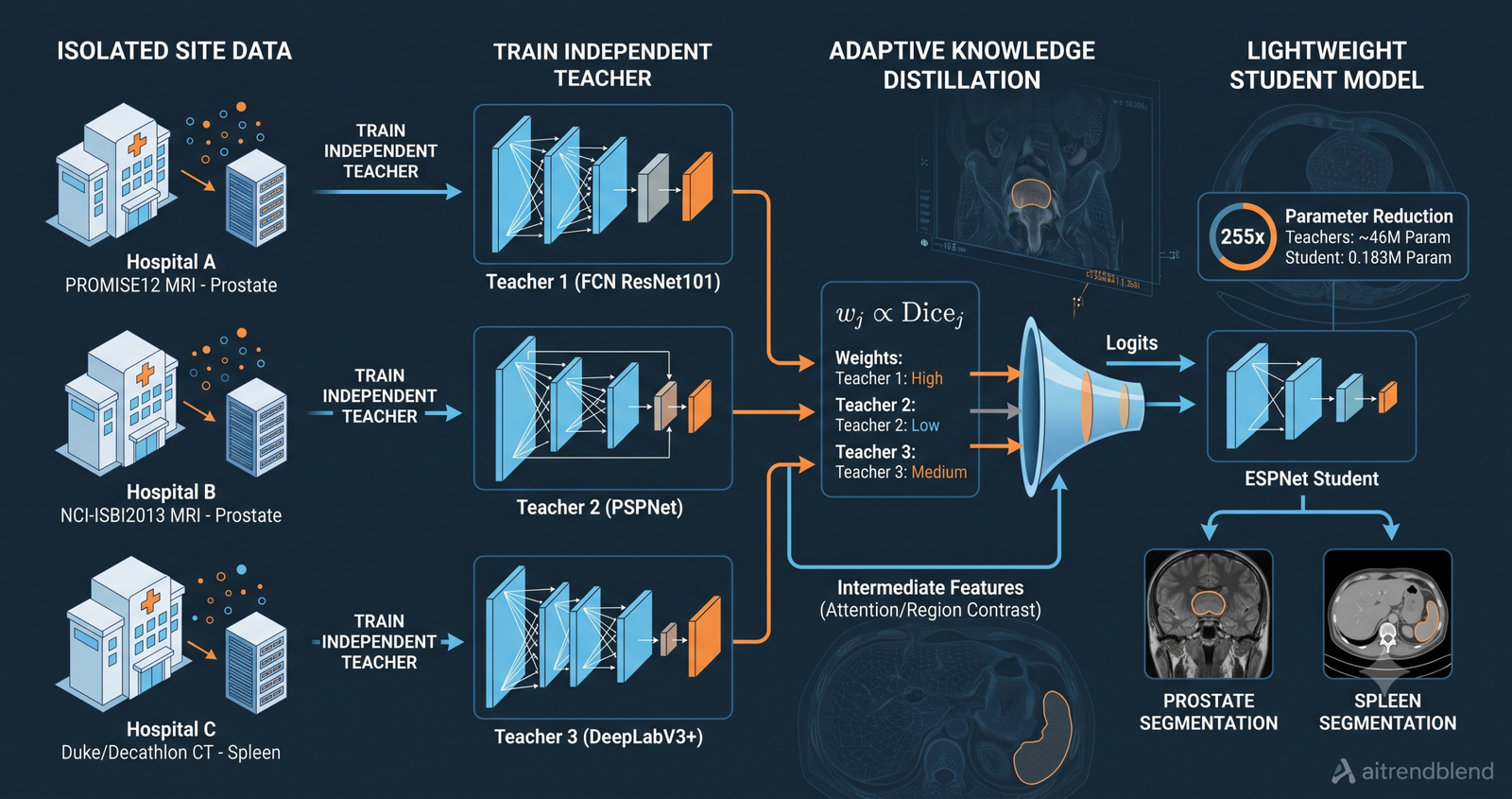
- The framework trains one teacher model per data source on limited, institution-specific data, then transfers their combined knowledge to a student using an adaptive weighting mechanism that adjusts each teacher’s contribution based on its per-batch performance.
- Three student networks tested (ENet, ESPNet, and MobileNetV2) all improve over their baselines on both prostate MRI and spleen CT segmentation after distillation, with the most compact student (ESPNet at 0.183 million parameters) reaching a dice score of 0.877 on spleen with dual-teacher distillation.
- The spleen multi-teacher result is markedly stronger than the prostate one. MobileNetV2 improves by 14.1% on spleen (0.714 to 0.855) versus 6.4% on prostate (0.784 to 0.848), a gap the paper attributes to the greater distribution difference between the Duke and Decathlon spleen sources.
- The adaptive weight for each teacher is proportional to its dice loss on the current batch, meaning a teacher that struggles with a given input gets higher weight rather than lower. The paper does not formally test the inverse weighting direction, which is a genuine gap in the ablation study.
- Against seven published knowledge distillation methods, the framework’s multi-teacher configuration reaches the highest dice scores on both prostate (0.869) and spleen (0.911), beating the nearest multi-teacher baseline AMTML-KD by 2.8% and 7.5% respectively.
- All experiments are retrospective on public benchmarks with augmented 2D slices from 3D volumes. No prospective clinical validation has been conducted.
The data problem that makes medical AI hard to deploy
A model trained to segment the prostate in MRI scans from one institution routinely fails when presented with scans from another hospital that uses a different scanner, a different field strength, or a different slice thickness. This is not a hypothetical concern, it is the standard outcome when clinical AI systems are applied outside their training distribution. The principled solution is to train on data from multiple sites, but the principled way of doing that while respecting patient privacy is not obvious.
The typical workaround in research papers is to pretend the privacy constraint does not exist, pool all available data, and train one large model. That approach produces good numbers on benchmarks but is often not reproducible in deployment because the data sharing agreements required to actually pool patient scans from multiple hospitals take months to negotiate and may never be granted at all.
Knowledge distillation offers a different path. If each institution trains its own model independently on its own data, and then the learned weights of those models are shared rather than the patient scans, the privacy constraint is substantially relaxed. Raw images stay on-site. What travels is the distilled function the model has learned. A student network that learns from the outputs and intermediate features of multiple such teachers can absorb a broader range of scan protocols and patient populations without any institution’s data ever leaving its firewall.
The paper takes this idea further than previous work by addressing two specific gaps. Earlier multi-teacher distillation methods either averaged the teachers’ contributions equally or used fixed weights determined before training, neither of which adapts to the difficulty of individual inputs. This framework computes adaptive weights dynamically at each training step based on how each teacher performs on the current batch.
The three-level distillation design
The knowledge transfer operates at two levels simultaneously, and the segmentation loss provides a third training signal that anchors the student to the ground truth labels.
Temperature-scaled logit distillation
At the output level, the student is asked to match the teacher’s softmax probability distribution, scaled by a temperature parameter that smooths the distribution and exposes more information in the relative probabilities between classes.
The transfer of these temperature-smoothed probabilities is measured by KL-divergence between the student and teacher distributions across all pixels in the segmentation map.
Where N equals the total number of pixels and \(p^s_i\), \(p^t_i\) are the student’s and teacher’s probability at the i-th pixel.
Intermediate feature distillation with attention transfer and region contrast
At the feature map level, the student is trained to replicate the spatial attention patterns of the teacher and to match the contrast between foreground and background regions that the teacher has learned to detect. The attention transfer loss takes the absolute value of each neuron’s activation, sums along the channel dimension to produce a spatial attention map, and then measures the normalized distance between the student’s and teacher’s maps.
Where \(rc^s_i\) and \(rc^t_j\) are region contrast vectors from the i-th and j-th layers of the student and teacher respectively, capturing how each network separates foreground tissue from background at that feature resolution. Attention transfer helps the student learn where to look. Region contrast teaches it what the boundary between tumor and surrounding tissue looks like in feature space.
Segmentation loss
The student’s output mask is also compared directly to the ground truth using a combination of Dice loss and Lovász-Softmax loss. Lovász-Softmax is particularly suited to segmentation tasks because it directly optimizes the intersection-over-union objective, which handles class imbalance better than cross-entropy when the foreground region occupies only a small fraction of the image.
The three losses combine into a single training objective.
The adaptive weighting mechanism for multiple teachers
When more than one teacher is present, the framework needs a principled way to combine their contributions. The paper’s answer is to weight each teacher’s contribution by its current dice loss on the batch, normalized so all weights sum to one.
Where y is the ground truth mask and \(p^{t_j}\) is teacher j’s prediction. The weighted teacher prediction \(p^t_i\) used in the KL-divergence loss is then \(\sum_j w_j \, p^{t_j}\), and the intermediate loss is correspondingly weighted as \(\sum_j w_j \, \mathcal{L}_{Mid}(t_j, s)\).
Experimental setup
The prostate dataset comes from three public sources combined into one split: PROMISE12, NCI-ISBI2013, and I2CVB, totaling 116 patients and 1,740 MRI slices with segmentation masks. For single-teacher distillation the full 80% training split was used. For multi-teacher distillation the training split was divided into three roughly equal subsets of 1,095, 1,113, and 638 slices, with one teacher trained on each. The three teachers for prostate were DeepLabV3+, FCN with ResNet101 as backbone, and PSPNet, each trained on its own subset.
The spleen dataset merges Decathlon (41 training CT volumes) and Duke DSDS (69 patients with chronic liver disease and portal hypertension scanned in axial CT). These two sources come from institutions with substantially different patient populations, acquisition protocols, and scanners. For dual-teacher distillation, the first teacher trained on Decathlon data and the second on Duke data. The top two teachers from the single-teacher experiments, DeepLabV3+ and FCN ResNet101, were selected for this role.
All images were preprocessed to a common canvas size, background removed with Otsu’s method, inverted, and resized to 170 by 242 pixels then center-cropped to 150 by 220. Extensive augmentation was applied including random rotation up to plus or minus 90 degrees, scaling, flipping, elastic transforms, brightness and contrast adjustment, and coarse dropout. Three student networks represented a range of parameter budgets. ESPNet at 0.183 million parameters and 1.27 GFLOPs sits at one extreme. ENet at 0.353 million parameters and 2.2 GFLOPs is in the middle. MobileNetV2 at 2.23 million parameters and 19.84 GFLOPs is the heaviest student, though still far lighter than the smallest teacher (PSPNet at 46.71 million parameters). Training ran for 100 epochs on a GeForce RTX 3080 Ti using the Adam optimizer with a cyclic learning rate schedule.
What the results actually show
Single-teacher distillation
All three students improve substantially across all teacher and dataset combinations. The most informative single number from the prostate results is ESPNet distilled from FCN ResNet101, which climbs from a baseline dice of 0.752 to 0.843, a gain of 12.1 percentage points, while the teacher itself sits at 0.901. The student reaches roughly 94% of the teacher’s performance at less than one half of one percent of its parameter count. Table 3 of the paper provides the full detail.
| Network | Prostate dice w/o | Prostate dice best w/ | Spleen dice w/o | Spleen dice best w/ |
|---|---|---|---|---|
| DeepLabV3+ (teacher) | 0.891 | — | 0.933 | — |
| FCN ResNet101 (teacher) | 0.901 | — | 0.945 | — |
| ENet (student) | 0.800 | 0.859 | 0.808 | 0.848 |
| ESPNet (student) | 0.752 | 0.843 | 0.773 | 0.840 |
| MobileNetV2 (student) | 0.784 | 0.853 | 0.714 | 0.802 |
FCN ResNet101 consistently outperforms the other three teacher architectures across every student and both datasets. The VOE metric (where lower is better) falls meaningfully for every combination, with ESPNet’s VOE dropping from 0.412 to 0.129 on prostate when distilled from FCN ResNet101, reflecting a substantially better delineation of the prostate boundary.
Multi-teacher distillation, where the gap between prostate and spleen is the story
| Network | Prostate baseline | Prostate w/ multi | Spleen baseline | Spleen w/ multi |
|---|---|---|---|---|
| ENet | 0.800 | 0.839 | 0.808 | 0.911 |
| ESPNet | 0.752 | 0.834 | 0.773 | 0.877 |
| MobileNetV2 | 0.784 | 0.848 | 0.714 | 0.855 |
The spleen numbers are dramatically stronger than the prostate ones, and this is the result that deserves the most careful reading. On prostate, the multi-teacher gain over baseline ranges from 3.9% to 8.2%. On spleen, it ranges from 10.3% to 14.1%. The paper explains this through the nature of the data sources. The Duke and Decathlon spleen datasets come from two entirely different institutions with different acquisition devices, leading to a large distribution gap between them. When two teachers are each trained on one of these maximally different sources, their combined knowledge covers a much broader region of the input space than either could cover alone, and the student’s performance reflects that coverage. The prostate dataset, though also multi-site, was collected with more consistent protocols across its three sources, so the benefit of diversity is proportionally smaller.
This observation has a direct practical implication. Multi-teacher distillation is most valuable when the contributing data sources are genuinely heterogeneous. An institution planning to deploy this framework should expect larger gains when it partners with sites that use different scanner brands and field strengths, and more modest gains when the partner sites are closely aligned in acquisition protocol.
“Our objective is not to enable the student to achieve higher performance by combining multiple teachers compared to learning from a single teacher.” Ben Loussaief et al., University Rovira i Virgili, Knowledge-Based Systems 2025
That quotation from Section 4.4.2 of the paper is worth holding alongside the spleen results. The authors are being appropriately careful. Multi-teacher distillation is not a mechanism for simply adding more training signal. It is a mechanism for enabling a model to generalize across diverse data distributions while the underlying patient data remains partitioned by site. On spleen, that goal is demonstrably achieved. On prostate, the gains over single-teacher are smaller, which is consistent with the paper’s stated objective rather than in tension with it.
Comparison with published KD methods
| Method | Prostate dice | Spleen dice |
|---|---|---|
| FCN ResNet101 (teacher ceiling) | 0.901 | 0.945 |
| ENet (student baseline) | 0.800 | 0.808 |
| Hinton KD (2014) | 0.765 | 0.811 |
| Attention Transfer (AT) | 0.816 | 0.822 |
| EMKD | 0.829 | 0.813 |
| CIRKD | 0.826 | 0.824 |
| ProtoKD | 0.770 | 0.846 |
| AMTML-KD (prior multi-teacher) | 0.841 | 0.836 |
| Ours single teacher | 0.859 | 0.848 |
| Ours multi teacher | 0.869 | 0.911 |
The comparison is conducted under identical conditions across all methods, which is the minimum required for a fair reading of the table. The framework’s single-teacher configuration already beats all seven baselines on prostate, and the multi-teacher configuration extends that lead. The most notable gap is on spleen, where AMTML-KD (the closest published multi-teacher baseline) reaches 0.836 and the proposed framework reaches 0.911, a difference of 7.5 percentage points. This is a large margin for a segmentation benchmark, though the paper uses a relatively small test set and the difference should be confirmed on larger independent cohorts before drawing strong conclusions about clinical applicability.
Clinical translation gap
The distance between these benchmark results and a deployed clinical tool is substantial, and it is worth describing concretely rather than in general terms.
Every segmentation result in the paper comes from retrospective data, meaning scans that were originally acquired for clinical purposes and later annotated for research. The model was trained and tested on 2D slices extracted from 3D volumes after preprocessing and augmentation. Real clinical deployment would involve the full 3D volume, potentially acquired on a scanner not represented in the training data, with no guarantee that the preprocessing pipeline would produce the same intensity distributions the model expects.
The prostate dataset of 116 patients spans three public research datasets. The spleen dataset spans 61 Decathlon volumes and 69 Duke volumes. These numbers are modest for a clinical benchmark and substantially smaller than what prospective validation trials typically require to establish safety and efficacy. In the European Union, software as a medical device that makes diagnostic claims falls under the Medical Device Regulation, which requires clinical evidence generated under the regulation’s own standards. In the United States, the FDA’s oversight of software-based medical imaging tools (classified under 510k or De Novo pathways depending on the specific claim) requires clinical studies that go well beyond retrospective benchmark comparisons.
The paper’s framework is also evaluated only on prostate MRI and abdominal spleen CT. Generalizing to other organs, other imaging modalities such as ultrasound or PET, or other pathological conditions has not been demonstrated and should not be assumed. The adaptive weighting mechanism and the distillation architecture are modality-agnostic in principle, but performance would need to be verified independently for each new application.
Clinical limitations
- The framework was tested on two organs (prostate and spleen) and two modalities (MRI and CT). Extension to ultrasound, X-ray, PET, or other organs has not been demonstrated and should not be assumed without separate experiments.
- The prostate dataset uses 116 patients across three public research collections. The spleen dataset uses approximately 130 CT volumes from two sources. Both are small relative to typical prospective clinical validation cohorts, and results may not generalize to broader patient populations, demographic groups, or pathological subtypes not well represented in these collections.
- The paper’s privacy argument, that patient data stays on-site because only model weights travel, is compelling but not formally analyzed. No adversarial reconstruction attack against the teacher weights was attempted, and the paper does not claim formal differential privacy guarantees.
- The adaptive weight formula (proportional to dice loss, not inverse) was not ablated against competing weighting strategies. The paper presents it as the proposed mechanism but does not demonstrate it is the optimal design through comparison.
- Qualitative results in Figures 4 through 7 show that multi-teacher distillation occasionally produces worse segmentation than single-teacher on individual cases (visible in Figure 5, row 3), which the paper acknowledges as pointing to the need for further enhancement of the multi-teacher scheme.
- No prospective clinical validation has been conducted. The system has not been tested on patients whose outcomes depended on the segmentation, and no regulatory approval of any kind is described. This paper represents a research prototype.
A reference PyTorch implementation
The code below is an independent educational reconstruction of the adaptive multi-teacher distillation framework described in the paper, written from the method description and equations. It is not the authors’ released code. The smoke test uses random tensors rather than real medical images. You can read the full paper here.
# adaptive_multiteacher_kd.py
# Independent educational implementation of the adaptive multi-teacher KD framework.
# Source paper: Ben Loussaief, Rashwan, Ayad, Khalid, Puig.
# Knowledge-Based Systems 315 (2025) 113196. DOI 10.1016/j.knosys.2025.113196
# Not the authors' released code. Written from method description and equations.

import torch
import torch.nn as nn
import torch.nn.functional as F


# ──────────────────────────────────────────────────────────────────────────────
# Attention Transfer loss (Zagoruyko & Komodakis 2017, used as AT_loss)
# Each feature map f of shape (B, C, H, W) is reduced to a spatial attention
# map by summing absolute activations along the channel dimension.
# ──────────────────────────────────────────────────────────────────────────────

class AttentionTransferLoss(nn.Module):
    """Compute AT loss between student and teacher feature maps.

    Matches equation 3 in the paper: ||norm(at_s) - norm(at_t)||_1
    where at is the channel-wise sum of absolute feature activations.
    """
    def forward(self, f_student, f_teacher):
        # f_student, f_teacher: (B, C, H, W) feature maps
        at_s = f_student.abs().sum(dim=1, keepdim=True)  # (B, 1, H, W)
        at_t = f_teacher.abs().sum(dim=1, keepdim=True)
        # Resize student map to match teacher spatial resolution if needed
        if at_s.shape != at_t.shape:
            at_s = F.interpolate(at_s, size=at_t.shape[-2:], mode="bilinear", align_corners=False)
        diff = at_s - at_t
        norm_diff = diff / (diff.norm(dim=[2, 3], keepdim=True) + 1e-8)
        return norm_diff.abs().mean()


# ──────────────────────────────────────────────────────────────────────────────
# Region contrast loss (based on Qin et al. 2021, used in MidLoss)
# Compares region-level feature contrast between foreground and background
# to transfer spatial boundary knowledge from teacher to student.
# ──────────────────────────────────────────────────────────────────────────────

class RegionContrastLoss(nn.Module):
    """Region contrast vectors derived from the segmentation mask.

    For each sample, compute the mean feature vector in the foreground (mask=1)
    and background (mask=0) regions separately. The L2 distance between the
    student and teacher contrast vectors forms the region contrast loss.
    This matches the rc term in equation 4 of the paper.
    """
    def forward(self, f_student, f_teacher, mask):
        # f_student, f_teacher: (B, C, H, W)
        # mask: (B, 1, H, W) with values in {0, 1} at the same spatial resolution
        B, C, H, W = f_student.shape
        if mask.shape[-2:] != (H, W):
            mask = F.interpolate(mask.float(), size=(H, W), mode="nearest")
        mask = mask.expand(-1, C, -1, -1)  # (B, C, H, W)
        fg_mask = mask
        bg_mask = 1.0 - mask

        def region_mean(feat, m):
            denom = m.sum(dim=[2, 3], keepdim=True).clamp(min=1.0)
            return (feat * m).sum(dim=[2, 3], keepdim=True) / denom

        rc_s_fg = region_mean(f_student, fg_mask)
        rc_s_bg = region_mean(f_student, bg_mask)
        rc_t_fg = region_mean(f_teacher, fg_mask)
        rc_t_bg = region_mean(f_teacher, bg_mask)

        loss_fg = F.mse_loss(rc_s_fg, rc_t_fg)
        loss_bg = F.mse_loss(rc_s_bg, rc_t_bg)
        return loss_fg + loss_bg


# ──────────────────────────────────────────────────────────────────────────────
# Dice loss (used for segmentation and adaptive weight computation)
# ──────────────────────────────────────────────────────────────────────────────

def dice_loss(pred, target, smooth=1.0):
    """Soft Dice loss. Equation 8 in the paper (Dice similarity coefficient).

    pred  : (B, C, H, W) probability map (after softmax or sigmoid)
    target: (B, 1, H, W) or (B, H, W) binary ground truth mask
    Returns a scalar loss in [0, 1], where 0 means perfect overlap.
    """
    if target.dim() == 3:
        target = target.unsqueeze(1)
    # Use the foreground channel (index 1) of a two-class prediction
    pred_fg = pred[:, 1:, :, :] if pred.shape[1] > 1 else pred
    target_f = target.float()
    intersection = (pred_fg * target_f).sum(dim=[1, 2, 3])
    union = pred_fg.sum(dim=[1, 2, 3]) + target_f.sum(dim=[1, 2, 3])
    dice = (2 * intersection + smooth) / (union + smooth)
    return (1.0 - dice).mean()


# ──────────────────────────────────────────────────────────────────────────────
# Adaptive multi-teacher distillation loss
# Implements equation 7 and the adaptive weight formula in Section 3.3
# ──────────────────────────────────────────────────────────────────────────────

class AdaptiveMultiTeacherKDLoss(nn.Module):
    """Compute the full adaptive multi-teacher KD loss.

    For each batch, computes adaptive weights w_j for each teacher
    based on their dice loss on the current batch (equation in Section 3.3).
    The combined teacher prediction and combined intermediate loss are
    then used to compute the KD objective (equation 6).

    Parameters
    ----------
    alpha : float
        Weight on the intermediate distillation loss. Paper uses 0.1.
    beta : float
        Weight on the KL divergence loss. Paper uses 0.1.
    alpha_seg : float
        Weight on the Dice component of SegLoss. Paper uses 0.2.
    alpha_lov : float
        Weight on the Lovász component of SegLoss. Paper uses 0.3.
    temperature : float
        Softmax temperature λ for logit distillation. Controls softness of targets.
    """

    def __init__(self, alpha=0.1, beta=0.1,
                 alpha_seg=0.2, alpha_lov=0.3, temperature=4.0):
        super().__init__()
        self.alpha = alpha
        self.beta = beta
        self.alpha_seg = alpha_seg
        self.alpha_lov = alpha_lov
        self.temperature = temperature
        self.at_loss = AttentionTransferLoss()
        self.rc_loss = RegionContrastLoss()

    def _kl_divergence(self, p_student, p_teacher):
        """KL divergence summed over classes, averaged over pixels."""
        log_s = F.log_softmax(p_student / self.temperature, dim=1)
        soft_t = F.softmax(p_teacher / self.temperature, dim=1)
        return F.kl_div(log_s, soft_t, reduction="batchmean") * (self.temperature ** 2)

    def _mid_loss_pair(self, feat_s, feat_t, mask):
        """Intermediate distillation loss between one teacher and the student."""
        at = self.at_loss(feat_s, feat_t)
        rc = self.rc_loss(feat_s, feat_t, mask)
        return at + rc

    def _compute_adaptive_weights(self, teacher_logits, ground_truth):
        """Equation from Section 3.3: w_j = DiceLoss(p_tj, y) / sum_k DiceLoss(p_tk, y)

        Note: teachers with higher dice loss get higher weight (see article
        for discussion of this design choice).
        """
        dice_losses = []
        for logits_j in teacher_logits:
            prob_j = F.softmax(logits_j, dim=1)
            dl = dice_loss(prob_j, ground_truth)
            dice_losses.append(dl)

        total = sum(dice_losses) + 1e-8
        weights = [dl / total for dl in dice_losses]
        return weights

    def forward(
        self,
        student_logits,      # (B, C, H, W) raw logits from student
        student_feat,        # (B, Cs, Hs, Ws) intermediate feature from student
        teacher_logits_list, # list of n tensors, each (B, C, H, W)
        teacher_feat_list,   # list of n tensors, each (B, Ct, Ht, Wt)
        ground_truth,        # (B, 1, H, W) or (B, H, W) binary mask
    ):
        if ground_truth.dim() == 3:
            ground_truth = ground_truth.unsqueeze(1)

        # Step 1: Segmentation loss (student vs. ground truth)
        student_prob = F.softmax(student_logits, dim=1)
        seg = dice_loss(student_prob, ground_truth)
        # Note: Lovász-Softmax requires a third-party package (pip install lovasz-losses)
        # For the smoke test we use dice only as a proxy for SegLoss
        seg_loss = self.alpha_seg * seg

        # Step 2: Compute adaptive weights for each teacher
        weights = self._compute_adaptive_weights(teacher_logits_list, ground_truth)

        # Step 3: Weighted teacher logits for KL divergence
        combined_teacher_logits = sum(
            w * logits
            for w, logits in zip(weights, teacher_logits_list)
        )
        kl = self._kl_divergence(student_logits, combined_teacher_logits)

        # Step 4: Weighted intermediate distillation loss across all teachers
        mid = sum(
            w * self._mid_loss_pair(student_feat, feat_t, ground_truth)
            for w, feat_t in zip(weights, teacher_feat_list)
        )

        # Step 5: Total KD loss — equation 6 in the paper
        total = seg_loss + self.alpha * mid + self.beta * kl
        return total, {
            "seg": seg_loss.item(),
            "mid": mid.item() if isinstance(mid, torch.Tensor) else float(mid),
            "kl": kl.item(),
            "weights": [w.item() if isinstance(w, torch.Tensor) else float(w) for w in weights],
        }


# ──────────────────────────────────────────────────────────────────────────────
# Minimal teacher and student stubs for the smoke test
# (Real use would substitute DeepLabV3+, FCN ResNet101, PSPNet as teachers
# and ESPNet, ENet, or MobileNetV2 as students)
# ──────────────────────────────────────────────────────────────────────────────

class TinySegNet(nn.Module):
    """Minimal two-class segmentation network for smoke testing."""
    def __init__(self, in_ch=1, n_classes=2, feat_ch=16):
        super().__init__()
        self.enc = nn.Sequential(
            nn.Conv2d(in_ch, feat_ch, 3, padding=1), nn.ReLU(inplace=True),
            nn.Conv2d(feat_ch, feat_ch, 3, padding=1), nn.ReLU(inplace=True),
        )
        self.head = nn.Conv2d(feat_ch, n_classes, 1)

    def forward(self, x):
        feats = self.enc(x)
        return self.head(feats), feats


# ──────────────────────────────────────────────────────────────────────────────
# Smoke test: confirms shapes and gradient flow are correct end to end
# ──────────────────────────────────────────────────────────────────────────────

def smoke_test(n_teachers=2):
    device = torch.device("cuda" if torch.cuda.is_available() else "cpu")
    B, H, W = 2, 64, 64

    # Build student and teachers
    student = TinySegNet(in_ch=1, feat_ch=8).to(device)
    teachers = [TinySegNet(in_ch=1, feat_ch=16).to(device) for _ in range(n_teachers)]
    for t in teachers:
        t.eval()

    kd_loss_fn = AdaptiveMultiTeacherKDLoss(
        alpha=0.1, beta=0.1, alpha_seg=0.2, temperature=4.0
    ).to(device)
    optimizer = torch.optim.Adam(student.parameters(), lr=1e-3)

    x = torch.randn(B, 1, H, W, device=device)
    gt = (torch.rand(B, 1, H, W, device=device) > 0.7).float()

    # Teacher forward passes (no grad)
    teacher_logits_list, teacher_feat_list = [], []
    with torch.no_grad():
        for t in teachers:
            logits_t, feats_t = t(x)
            teacher_logits_list.append(logits_t)
            teacher_feat_list.append(feats_t)

    # Student forward pass (with grad)
    optimizer.zero_grad()
    student_logits, student_feats = student(x)

    total_loss, components = kd_loss_fn(
        student_logits, student_feats,
        teacher_logits_list, teacher_feat_list,
        gt,
    )
    total_loss.backward()
    optimizer.step()

    print(f"Smoke test passed with {n_teachers} teacher(s).")
    print(f"Total KD loss: {total_loss.item():.4f}")
    print(f"  SegLoss: {components['seg']:.4f}")
    print(f"  MidLoss: {components['mid']:.4f}")
    print(f"  KL loss: {components['kl']:.4f}")
    print(f"  Teacher weights: {[f'{w:.3f}' for w in components['weights']]}")
    print(f"  Student output shape: {student_logits.shape}")


if __name__ == "__main__":
    smoke_test(n_teachers=2)   # dual teacher: matches spleen experiment
    smoke_test(n_teachers=3)   # trio teacher: matches prostate experiment
Conclusion
The framework described in this paper addresses a genuinely difficult problem in clinical AI deployment: how to train a model that generalizes across multiple medical imaging sites when the practical and legal barriers to pooling patient data are high. By training separate teacher models on isolated institutional datasets and transferring their combined expertise to a single lightweight student, the approach gives the student access to the diversity of multiple data sources without any institution’s patient scans ever leaving that institution’s storage systems. The distillation process carries the information, not the data.
The adaptive weighting mechanism is the technical contribution that distinguishes this approach from earlier multi-teacher frameworks that average contributions equally or use fixed performance-based weights. Whether weighting teachers by their dice loss in the direction the paper proposes (higher loss gets higher weight) is the optimal direction is an open question the paper does not fully answer, and it represents an area where practitioners adapting this framework should invest experimental effort before committing to the design.
The spleen results are the most compelling in the paper, and they are compelling for a reason that extends beyond a single experiment. The large performance gap between single-teacher and multi-teacher distillation on spleen, compared to the modest gap on prostate, appears to track directly with how different the contributing data sources actually are from each other. Duke and Decathlon differ in institution, scanner, and patient population in ways that the three prostate sources do not. If that relationship holds in other applications, it gives practitioners a practical guide for predicting when multi-teacher distillation is likely to add the most value.
The efficiency story is also worth taking seriously on its own terms. ESPNet at 0.183 million parameters is a model that can run on hardware that most hospital radiology departments already have. A dice score of 0.877 on spleen segmentation after distillation, achieved on a model that requires 1.27 GFLOPs per inference pass, opens the door to segmentation pipelines that are feasible on workstation hardware rather than requiring data center GPU infrastructure. Whether 0.877 is clinically sufficient depends on how tightly the segmentation result is integrated into clinical decision-making and on expert radiological review, which neither this article nor the underlying paper can substitute for.
The path from these benchmark results to a validated clinical tool runs through prospective validation studies, regulatory assessment, and expert clinical evaluation that the paper does not attempt and that no benchmark alone can provide. What this research does establish is that the architectural approach is sound, the privacy-respecting data partitioning works as intended, and the performance gains from multi-source multi-teacher distillation are real and reproducible on public benchmarks. Those are the right questions for a research paper to answer. The clinical questions are the right ones for a subsequent, well-designed trial.
Frequently asked questions
What is multi-teacher knowledge distillation in the context of this paper
It is a training approach where multiple teacher models, each trained on data from a different hospital or imaging site, simultaneously guide a single lightweight student model. The student learns from the predictions and feature maps of all teachers together rather than from a single combined dataset, allowing it to absorb diverse scanning protocols without accessing any institution’s patient data directly.
How does the adaptive weighting mechanism work
At each training batch, the framework computes a dice loss for each teacher model against the ground truth mask. Each teacher’s weight is set proportional to its dice loss on that batch, normalized so all weights sum to one. The paper’s design means a teacher that performs less well on a given input receives higher weight, providing complementary information to the better-performing teachers. Whether this weighting direction is optimal over the inverse was not formally ablated in the paper.
Why are the spleen results so much stronger than the prostate results
The paper attributes this to the nature of the two data sources for spleen. The Decathlon and Duke datasets come from institutions with substantially different acquisition protocols, scanner hardware, and patient populations. When two teachers are each trained on one of these very different sources, their combined knowledge covers a broader distribution than a single teacher could. The prostate sources are also multi-site but more similar to each other in acquisition protocol, so the added diversity from multiple teachers is smaller.
Does this approach provide real patient data privacy protection
The framework substantially reduces privacy risk compared to pooling patient scans, because raw images stay at each institution and only learned model weights travel. The paper does not claim formal differential privacy guarantees and does not test adversarial weight inversion attacks against the teacher weights. The privacy benefit is practically meaningful but should not be equated with a mathematically proven privacy guarantee.
What lightweight student architecture should a practitioner choose
ESPNet at 0.183 million parameters and 1.27 GFLOPs is the most efficient option tested and achieves competitive dice scores after distillation. ENet at 0.353 million parameters tends to reach slightly higher absolute dice. MobileNetV2 at 2.23 million parameters offers a larger capacity student that may be preferable if the deployment device has more GPU memory. The choice should depend on the inference hardware available and the acceptable trade-off between model size and segmentation accuracy for the specific clinical task.
Is this approach ready for clinical use
No. The experiments are retrospective on public research datasets totaling 116 prostate patients and approximately 130 spleen CT volumes. No prospective clinical validation has been conducted, and the framework has not received regulatory review or approval in any jurisdiction. A clinician or clinical AI team considering adapting this approach should treat it as a research prototype that requires independent prospective validation before any clinical deployment decision.
Read the full method, ablation context, and visual segmentation comparisons in the source paper.