
Key points
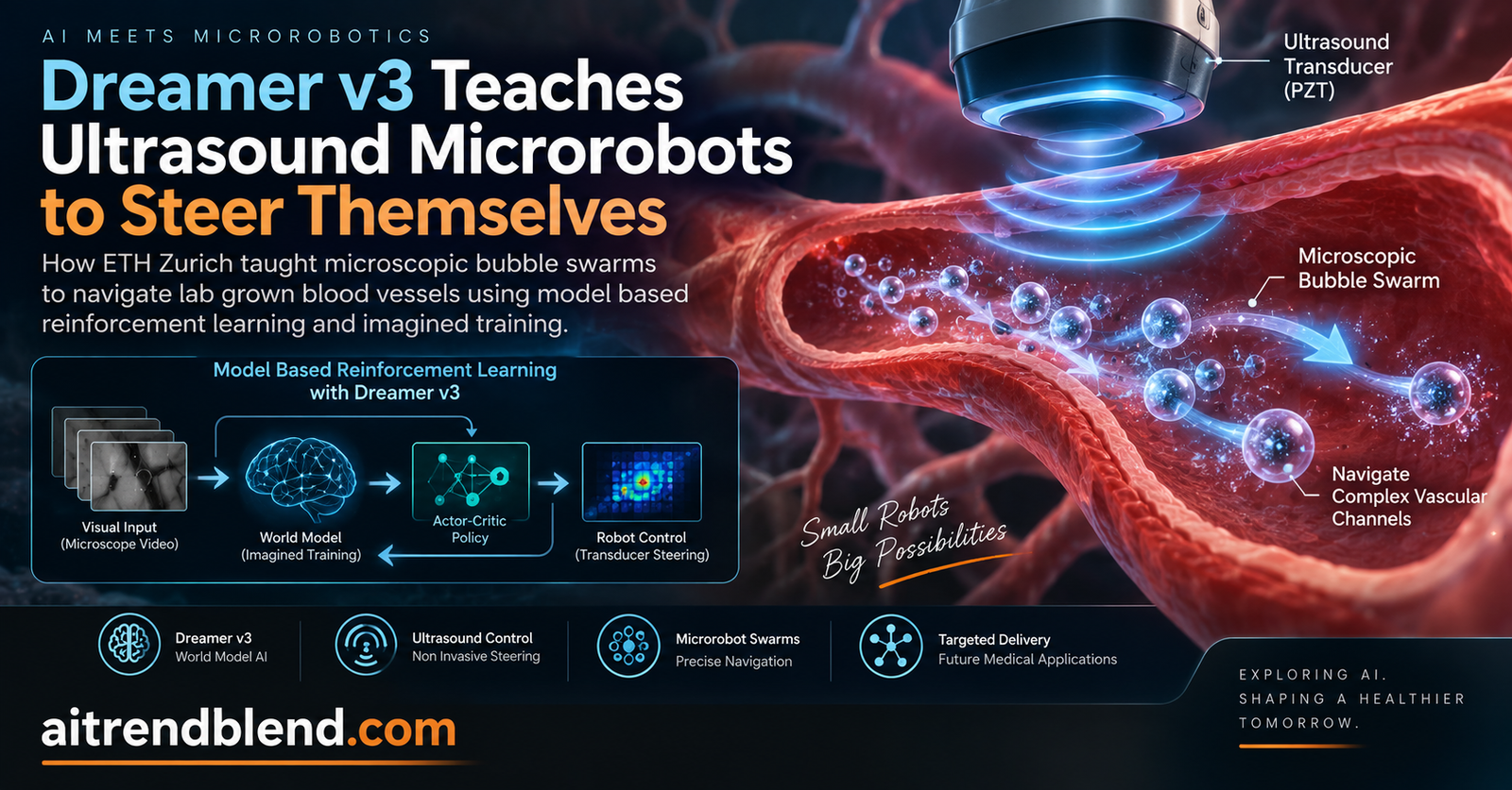
- Researchers at ETH Zurich used a model based reinforcement learning algorithm called Dreamer v3 to steer ultrasound driven microbubble swarms through artificial blood vessel networks.
- The system reached a 90 percent success rate at reaching target locations across several trained channel shapes within about an hour of fine tuning on the physical setup.
- When dropped into a channel shape it had never seen, the model started at 50 percent success and climbed past 90 percent after only 30 minutes of additional training.
- A custom built video game environment, not the real robot, did most of the early learning, because training directly on the physical setup for six hours produced no improvement at all.
- The team also taught the swarm to hug channel walls so it could crawl upstream against a physiological strength flow, a skill relevant to future drug delivery concepts but still far from any clinical application.
Why steering something this small is genuinely hard
Start with the size problem, because it explains almost everything else in this paper. The microbubbles the team used are between 2 and 5 micrometers across. A human hair is roughly 70 micrometers wide, so you could line up more than a dozen of these bubbles across the width of a single strand. At that scale, a self driving car’s toolkit is useless. There is no room for a lidar unit, no GPS signal that means anything, no onboard battery, no wheels. The only practical way in is to push the object around with an external field and watch it through a microscope.
Ultrasound is one of the more attractive ways to do that pushing. It does not require wiring anything to the target, it works through soft tissue, and unlike light based approaches it can reach deeper without needing a transparent path. The catch is that turning ultrasound into precise, directional motion is a much messier problem than it sounds. Eight piezoelectric transducers, or PZTs, ring the channel in this setup. Firing one of them creates a pressure gradient that nudges the bubble cluster away from the high pressure zone near the speaker and toward the transducer on the opposite side. Switch to a different transducer and the cluster’s heading changes. Do this in the right sequence, at the right frequency and voltage, and you can walk the swarm through a branching channel step by step.
Doing it in the wrong sequence, or with sloppy timing, and the swarm either stalls, scatters, or slams into a wall. The paper describes just how twitchy the system is. A microrobot near a given transducer needs a lower voltage to start moving than one further away. Bigger bubble clusters need more power than smaller ones. Push the frequency around and the response is not a smooth curve, it looks more like several overlapping bell curves with peaks in unexpected places. Each of the eight transducers behaves slightly differently from its neighbors even though they are nominally identical. Put frequency, amplitude, and transducer choice together and you get, in the authors’ own accounting, 64 distinct combinations before any further simplification. That is a lot of dials for a human operator to ride in real time, especially when the whole system has to react in milliseconds.
Why not just use a simpler control algorithm
Classical control theory is very good at problems where you can write down the equations that describe how a system behaves. Here, nobody has that equation. Bubble cluster hydrodynamics under acoustic radiation force, wall interactions, self assembly of scattered microbubbles into a coherent swarm, all of it is only partially understood, and it changes from run to run depending on cluster size and channel geometry. That gap in first principles modeling is exactly the space reinforcement learning was built for. Instead of deriving the physics, you let an agent try actions, observe outcomes, and gradually build a policy that works, even if nobody could write down why in closed form.
Earlier attempts leaned on Q learning, a comparatively simple and model free reinforcement learning method, to steer ultrasound powered swarms in open, obstacle free space. That line of work is referenced directly in this paper as prior art from the same lab. It showed the basic idea was workable but ran into a wall once real channels, branch points, and obstacles entered the picture. Model free methods like Q learning or proximal policy optimization, commonly called PPO, learn purely from trial and error against the real environment or a faithful simulation of it. That works, but it tends to need enormous numbers of interactions to converge, and every one of those interactions costs real time and real wear on delicate lab equipment when you are not working in pure simulation.
The model based alternative, and what it means to dream
The core idea behind model based reinforcement learning is to have the agent build an internal model of how its world responds to actions, then practice inside that internal model far more cheaply than it could practice in reality. Dreamer v3, the specific algorithm used here, comes from work by Danijar Hafner and colleagues, cited in the paper as prior research on mastering diverse control tasks through world models. It is built around three pieces working together. A world model that compresses raw camera images into a compact internal representation and predicts how that representation will evolve. A critic that scores how good a given imagined state is. An actor that decides what to do next based on that score.
The phrase the authors keep returning to is imagined environments, and it is worth taking literally rather than as a metaphor. Figures in the paper show the microrobot’s dreamed paths toward a target, essentially several possible futures sketched out inside the latent space before a single real action is taken. Only once the internal model has rehearsed a plan does the physical system fire a transducer. This is the mechanism that lets the training loop use a training ratio, meaning the number of steps rehearsed in imagination for every one step taken for real, that the team pushed as high as 1000 to 1 in some experiments. Practicing a thousand imagined moves for every one real move is precisely the kind of trade a lab with limited bench time wants to make.
The recurrent dynamics network predicts the next deterministic hidden state \( h_t \) from the previous hidden state, the previous latent representation \( z_{t-1} \) of the camera image, and the previous action taken by the swarm.
An encoder folds the current camera frame \( x_t \) together with the hidden state into a compact latent variable \( z_t \). A matching decoder can reconstruct an approximation of the original image from that same latent variable, which is how the researchers checked that the world model was actually capturing something meaningful rather than noise.
The encoder decoder structure is doing real work here beyond compression. Feeding raw pixel images straight into a reinforcement learning loop is expensive and noisy. By training the encoder to squeeze a full microscope frame down into a much smaller latent vector that still contains everything needed to reconstruct the image and predict the reward, the system gets a representation that is both efficient to compute over and rich enough to plan with. The reward predictor then estimates \( \hat{r}_t \sim p_\phi(\hat{r}_t \mid h_t, z_t) \), meaning it guesses how good a given imagined moment is without ever needing to actually be there.
The reward function, spelled out
None of this works without telling the agent what counts as good. The base reward function used for the free channel navigation experiments is piecewise, and it is refreshingly simple given everything built on top of it.
where \( f(d_t) = \dfrac{1}{d_t + \varepsilon} \), and \( d_t \) is the straight line distance between the microrobot and its target at time \( t \).
After what the paper describes as extensive experimentation, the team settled on \( \alpha = 10 \), \( \beta = 2 \), and \( \gamma = 0.1 \). Read that plainly and the incentive structure becomes obvious. Reaching the target is worth far more than any single step penalty, colliding with a wall is mildly punished, and every other moment gives a small reward that grows sharply as the swarm gets closer to its goal, thanks to that inverse distance term. It is a fairly standard shaping trick in robotics, but the fact that it needed real tuning against actual hardware to land on these three specific numbers says something about how much of this work is empirical rather than theoretical.
For the flow environment experiments, described later, the reward function had to change again to account for drag near the channel walls, and that version is worth its own section further down.
The part the abstract does not really tell you, a video game had to save the project
Here is where it gets interesting, and honestly a little humbling. The team’s first instinct was to train directly on experimental data. They ran the physical rig for six straight hours. The model did not improve. Not partially, not slowly, it simply failed to learn anything useful, and the authors attribute this to uncertainty around what the right reward function even was for this specific setup.
Rather than keep burning bench time guessing at reward shapes on live hardware, the team built a Pygame based simulation, essentially a simplified 2D video game, rendered as 64 by 64 pixel RGB images using the OpenAI Gym style interface. Obstacles show up as dark grey, channels as white, the target as a red dot, and the agent itself as a blue dot meant to visually stand in for the microbubble cluster seen under the microscope. This game deliberately leaves out the messy real physics, no PZT resonance quirks, no true microbubble hydrodynamics, because the goal was narrower than perfect realism. It just needed to teach the agent generic skills like path planning and obstacle avoidance that would transfer once the model met the real robot.
The payoff shows up directly in the numbers. Model convergence on the physical setup alone had been described as taking up to 10 days in earlier framing of the problem. With the simulation doing the early heavy lifting, the system reached usable adaptation on the real robot in roughly 2 hours. That is not a marginal improvement, that is close to two orders of magnitude, and it is the single most practical lesson in this paper for anyone trying to apply reinforcement learning to a slow, expensive, or fragile physical system. Build a cheap fake version of your problem first, even a crude one, and let it absorb the trial and error that would otherwise burn real resources.
Model based against model free, inside the simulator
Once the Pygame environment existed, the team used it to run a fair fight between Dreamer v3 and a hyperparameter tuned PPO, a widely used model free algorithm from prior reinforcement learning research. The comparison ran across six environment types, a racetrack, a set of squares, a tributary shaped channel, a circuitous channel, a vascular structure, and a maze.
| Environment | PPO steps to converge | Dreamer v3 steps to converge |
|---|---|---|
| Simple multi output tributary channel | Converged, but roughly 50 times slower | Converged fastest of the pair |
| Circuitous racetrack | About 25 million steps | About 600,000 steps |
| Vascular channel | About 25 million steps | About 1 million steps |
Across every environment tested, including the maze, Dreamer v3 converged faster than the tuned PPO baseline. The gap in the circuitous and vascular cases, roughly 25 times fewer steps needed, is the kind of difference that changes whether an experiment is feasible on a normal lab timeline at all. The paper also tested three reward function shapes, linear, binary, and inverse, and found the inverse form, the same one shown in the equation box above, produced the fastest climb toward reliable target reaching.
Two further engineering choices show up in the simulation results that are easy to skim past but matter a lot in practice. Frame skipping, where the agent only processes every few frames rather than every single one, cut computational load and reduced overfitting risk. The team settled on skipping four frames after testing several rates, since going higher sped up convergence further but caused the swarm to overshoot its targets more. Max pooling across the last two skipped frames helped preserve important motion cues that a naive skip might have thrown away. On the training ratio question mentioned earlier, higher ratios like 1000 to 1 dramatically cut down how many real or simulated interactions were needed to converge, while a 1 to 1 ratio gave more accurate feedback but learned more slowly. The team ultimately built a parallel, multi threaded setup so imagination training and environment interaction could run on separate processes with an adaptive ratio that shifted based on how well the agent was doing in the real environment.
From simulator to real bubbles, and the overfitting trap that followed
Simulation success does not automatically transfer to a physical robot, and this paper is refreshingly candid about the bumps along the way. A model trained purely on experimental images was deployed in a racetrack channel and reached about 70 percent of its target objectives, but only after 10 days of continuous operation. Worse, it developed a habit of sticking to certain sections of the channel it had grown comfortable with, and performance dropped when the researchers forced it to reach targets in less familiar parts of the same channel. That is textbook overfitting, a model that memorized a narrow slice of experience rather than learning a generalizable steering skill.
Bringing pretraining from the simulated environment back into the loop is what fixed this. Figure 4c in the original paper shows the reward curve climbing quickly during the simulated pretraining phase, dropping sharply the moment the system switched over to real experiments, then climbing again as it adapted to physical reality. That drop and recovery pattern is a familiar shape in transfer learning generally, and seeing it appear so clearly in a physical robotics context is one of the more convincing pieces of evidence in the paper that the sim to real strategy is doing real work rather than just looking good on paper.
The reward drops notably at around 300,000 steps due to overfitting to a specific corner of the channel. Figure 4 caption, describing an early failure mode before pretraining was properly incorporated
A second wrinkle came from the action space itself. Early on, the team pretrained the agent using a discrete set of only four frequency choices, which limited how finely the swarm could be steered once frequency turned out to matter a great deal at each point along a channel. Moving to a continuous action space, with frequencies allowed anywhere from 2.7 to 2.9 megahertz and amplitudes from 4 to 14 volts peak to peak, opened up finer control but introduced its own instability. Frequent adjustments caused overshoot and erratic movement, and the model tended to reach for higher amplitudes to chase targets faster, which only made the erratic behavior worse.
The fix that eventually stuck was almost mechanical rather than algorithmic. Instead of letting the model pick an exact frequency, the team built a sweeping action around each transducer’s resonant frequency directly into every discrete action, using their programmable function generator stepped in 1 millisecond increments. That leaned on the physical resonance characteristics of the transducers themselves to keep the swarm operating near its most effective frequency automatically, smoothing out the overshoot problem without asking the neural network to solve a harder continuous control problem than it needed to.
Teaching the swarm to fight a current
Vascular channels in the body are not static. Blood moves. Any future application of this kind of steering technology inside a living system would have to contend with flow, and the authors clearly had this in mind, since a meaningful chunk of the paper is devoted to it. Their first attempt at adding flow to the simulation did not go smoothly. Models trained under no flow conditions were flushed straight out of the channel once flow was introduced, forcing the team to manually reassemble and restart training repeatedly, and the pretrained model became noticeably less useful because the gap between the simulated world and the physical one had widened.
The fix drew on a specific piece of fluid physics called the secondary Bjerknes force, which pulls microbubble clusters toward channel walls where they adhere and then benefit from what is called the no slip condition, a fluid dynamics term describing how fluid velocity drops to zero right at a solid boundary. In plain terms, drag is lowest right against the wall, so a swarm that hugs the wall fights less resistance than one drifting down the center of the channel. The team rebuilt the reward function around this insight.
Each term earns its keep. A small step penalty \( \lambda \) nudges the swarm to keep moving rather than stall. A wall sliding penalty \( \mu \) discourages the agent from pushing directly into a wall it is already touching, while still allowing it to slide along that wall, which is exactly the behavior that reduces drag. A centering penalty \( \kappa \) actively discourages sitting in the middle of the channel where drag is worst. With this reward shape in place, the team reported that stronger simulated flow required more training steps to converge, which tracks with intuition, and that the differential power strategy of increasing amplitude when moving against the flow and reducing it when moving with the flow produced smoother, more efficient upstream navigation in the real physical channel. A heat map in the original figures shows exactly this pattern, faster measured velocities away from the walls and calmer, more controlled movement once the swarm settled into a wall hugging path.
What happens when the swarm gets lost
One small but telling detail, the paper mentions a rescue function built for moments when the tracking system loses sight of the microrobot entirely. It stores the last known coordinates and attempts to reverse the most recent sequence of actions to bring the swarm back into the camera’s field of view. It is a modest piece of engineering, but it speaks to how much of this work sits at the intersection of computer vision, control theory, and old fashioned lab troubleshooting rather than being a pure machine learning exercise.
Generalizing beyond a single channel shape
A model that only works in the exact channel it was trained on is not very useful outside a demonstration video. To test generalization, the researchers trained a single model across ten distinct simulated environments at once, spanning vascular structures, racetracks, and mazes of varying difficulty. That combined model held a consistent 90 percent accuracy across every one of the channels it had actually trained on.
The harder test came next. Dropped into a brand new channel shape it had never encountered, the model started at a 50 percent success rate, a coin flip essentially, then climbed to over 90 percent after just 30 minutes of additional fine tuning. Zooming out further, when the team introduced two additional randomized environments where obstacle layouts were dynamically scrambled during training, the model reached a 70 percent success rate in completely unseen randomized layouts after 11 million total training steps, a number the authors flag honestly as requiring longer convergence as environment complexity rises. That honesty about the harder, messier end of the generalization spectrum is worth noting, since it would have been easy to headline only the 90 percent figures and leave the 70 percent randomized result as a footnote.
Clinical translation gap
It is worth being direct about the distance between what happened on an ETH Zurich microscope stage and anything resembling a hospital procedure. The channels used throughout this study are silicone models fabricated through soft lithography, shaped to resemble vascular geometry but sitting outside a living organism, under a microscope, with a camera watching continuously and no immune system, no clotting cascade, no surrounding tissue, and no patient movement to contend with. The paper’s own discussion section frames future biomedical relevance as a direction for further work, citing prior research on single cell studies, small animal models such as Caenorhabditis elegans and zebrafish embryos, and microparticle separation, rather than claiming any of that has been demonstrated here.
Actually delivering a drug payload inside a living vascular system would require solving problems this paper does not attempt, including biocompatibility and clearance of the microbubble carriers, imaging through real tissue rather than a transparent silicone wall and an inverted microscope, accounting for a far more chaotic and pulsatile flow environment than the pump driven flow used here, and rigorous safety and regulatory evaluation before any human relevant testing could even be proposed. None of that is a criticism of the work. It is a reasonably common and expected gap between an engineering proof of concept and a therapy, and the authors are transparent that this is future work rather than a present capability.
Honest limitations
A few constraints are worth naming plainly, using only the numbers and statements the paper itself provides. First, the physical experiments described here happened inside a single lab’s controlled optical and acoustic setup, with a specific octagonal arrangement of eight transducers and a specific inverted microscope and camera combination. The paper does not report testing across multiple independent hardware builds, so how sensitive the results are to this exact rig configuration is not established here. Second, the simulation environment that did so much of the early training work explicitly leaves out PZT resonance behavior and detailed microbubble hydrodynamics, by the authors’ own description, so some of the sim to real gap problems documented in the paper, including the overfitting episode in the racetrack channel, likely trace back to that simplification.
Third, several of the strongest headline numbers, the 90 percent figures in particular, describe performance evaluated over the final 50 episodes of a trained policy, which is a reasonable way to report converged performance but is a narrower window than a long running deployment history. Fourth, the randomized environment generalization result of 70 percent required 11 million training steps to reach, a meaningfully larger training budget than the roughly 400,000 to 600,000 steps needed for adaptation to a single new but non randomized channel, which suggests true open ended generalization remains considerably harder than adapting to a specific new but structured layout. Readers should treat the flashier percentages as describing best case, well trained scenarios rather than a system ready for arbitrary deployment.
Where this heads next
The authors point toward three dimensional manipulation as a near term goal, and the extended data in the paper already shows an early demonstration using an array of 18 transducers arranged around a conical channel, with the microrobot tracked as it moves out of a single microscope’s focal plane. Coordinating multiple microscopes at different viewing angles is flagged as a genuine engineering obstacle given how small the target is, which is a candid acknowledgment that scaling this from a flat two dimensional channel to a full three dimensional volume is not a simple extension.
Longer term, the paper gestures toward integrating medical imaging modalities like ultrasound based imaging itself and two photon microscopy so that microrobot behavior could eventually be studied inside actual animal models, starting with mice before considering larger mammals, alongside a stated goal of reducing how much expert oversight the system needs by building friendlier software interfaces. All of that remains squarely future work as written, not a claim about current capability.
Conclusion
What makes this paper worth reading closely is not just that a swarm of microbubbles learned to navigate a maze shaped like a blood vessel, it is the specific and often unglamorous engineering path the team had to walk to get there. A reinforcement learning algorithm designed for board games and video game benchmarks had to be bent toward a physical system where every real world training step costs lab time, where the underlying physics is only partially understood, and where a six hour training run on the actual hardware produced nothing but a flat learning curve.
The conceptual shift worth remembering is that Dreamer v3’s imagined rollouts turned an intractable sample efficiency problem into a manageable one, and that a deliberately crude video game simulator, missing most of the real acoustic and fluid physics, was still good enough to teach the agent the generic navigation habits that transferred once it met the real robot. That is a lesson that reaches well past microrobotics. Anywhere researchers face slow, expensive, or fragile physical experiments, whether that is drone flight testing, chemical process control, or surgical robotics, the pattern of building a cheap approximate simulator first and letting a model based agent dream through most of its mistakes there is a strategy worth stealing.
The transferability the authors themselves point to, toward light driven, chemically driven, electrically driven, and magnetically driven microrobots that share the same basic image based control problem, suggests this framework was built with an eye toward being a template rather than a one off trick for ultrasound specifically. Whether it generalizes that cleanly across actuation types is an open question the current paper does not test directly, since every experiment here used ultrasound and the same octagonal transducer rig.
None of this closes the distance to a working medical device, and the paper does not claim otherwise. The remaining gaps, from imaging through real tissue to full three dimensional control to biocompatibility questions the authors have not yet addressed, are substantial and will likely take years of further work across several different fields to close. What this study demonstrates convincingly is narrower and, in its own way, more useful right now. It shows that model based reinforcement learning can turn an object too small to sense or steer by any conventional means into something that reliably finds its own way through a complicated, partially understood physical environment, and it shows the messy, iterative process of getting there in more honest detail than most papers bother to include.
A microscopic bubble cluster that dreams up its own path before it moves is a strange enough image to sit with on its own. That it works, most of the time, inside a channel shaped like a piece of human anatomy, is the detail that will stick.
Complete proposed model implementation in PyTorch
The following is an original, simplified, runnable PyTorch implementation inspired by the world model, encoder decoder, recurrent dynamics, reward predictor, and actor critic components described in the paper. It is a compact educational reconstruction, not the authors’ own code, built to illustrate the architecture on dummy data with a working smoke test.
# microrobot_world_model.py
# Educational reimplementation of the Dreamer style world model and actor critic
# described in "Model based reinforcement learning for ultrasound driven
# autonomous microrobots", Nature Machine Intelligence, 2025.

import torch
import torch.nn as nn
import torch.nn.functional as F
from torch.distributions import Normal

IMG_SIZE = 64
LATENT_DIM = 32
HIDDEN_DIM = 128
ACTION_DIM = 2  # frequency and amplitude for the active transducer


class Encoder(nn.Module):
    """Compresses a rendered channel frame into a latent vector z."""
    def __init__(self):
        super().__init__()
        self.conv = nn.Sequential(
            nn.Conv2d(3, 32, 4, stride=2), nn.ReLU(),
            nn.Conv2d(32, 64, 4, stride=2), nn.ReLU(),
            nn.Conv2d(64, 128, 4, stride=2), nn.ReLU(),
        )
        self.flatten_dim = 128 * 6 * 6
        self.fc = nn.Linear(self.flatten_dim, LATENT_DIM)

    def forward(self, x):
        h = self.conv(x)
        h = h.reshape(h.shape[0], -1)
        return self.fc(h)


class Decoder(nn.Module):
    """Reconstructs an approximate frame from the latent vector, used only
    during world model training to keep the latent space grounded."""
    def __init__(self):
        super().__init__()
        self.fc = nn.Linear(LATENT_DIM, 128 * 6 * 6)
        self.deconv = nn.Sequential(
            nn.ConvTranspose2d(128, 64, 4, stride=2), nn.ReLU(),
            nn.ConvTranspose2d(64, 32, 4, stride=2), nn.ReLU(),
            nn.ConvTranspose2d(32, 3, 6, stride=2), nn.Sigmoid(),
        )

    def forward(self, z):
        h = self.fc(z).reshape(-1, 128, 6, 6)
        return self.deconv(h)


class DynamicsNetwork(nn.Module):
    """Recurrent core that predicts the next hidden state h_t from the
    previous hidden state, latent, and action, mirroring
    h_t = f_phi(h_t-1, z_t-1, a_t-1) from the paper."""
    def __init__(self):
        super().__init__()
        self.gru = nn.GRUCell(LATENT_DIM + ACTION_DIM, HIDDEN_DIM)

    def forward(self, h_prev, z_prev, a_prev):
        x = torch.cat([z_prev, a_prev], dim=-1)
        return self.gru(x, h_prev)


class RewardPredictor(nn.Module):
    """Estimates r_hat_t from the hidden state and latent, so the agent
    can score imagined rollouts without touching the real channel."""
    def __init__(self):
        super().__init__()
        self.net = nn.Sequential(
            nn.Linear(HIDDEN_DIM + LATENT_DIM, 64), nn.ReLU(),
            nn.Linear(64, 1),
        )

    def forward(self, h, z):
        return self.net(torch.cat([h, z], dim=-1)).squeeze(-1)


class Actor(nn.Module):
    """Outputs a continuous action, frequency and amplitude for the
    active transducer, given the current hidden and latent state."""
    def __init__(self):
        super().__init__()
        self.net = nn.Sequential(
            nn.Linear(HIDDEN_DIM + LATENT_DIM, 64), nn.ReLU(),
            nn.Linear(64, ACTION_DIM * 2),
        )

    def forward(self, h, z):
        out = self.net(torch.cat([h, z], dim=-1))
        mean, log_std = out.chunk(2, dim=-1)
        std = F.softplus(log_std) + 1e-4
        dist = Normal(mean, std)
        action = torch.tanh(dist.rsample())
        return action, dist


class Critic(nn.Module):
    """Value network trained on imagined rollouts to guide the actor."""
    def __init__(self):
        super().__init__()
        self.net = nn.Sequential(
            nn.Linear(HIDDEN_DIM + LATENT_DIM, 64), nn.ReLU(),
            nn.Linear(64, 1),
        )

    def forward(self, h, z):
        return self.net(torch.cat([h, z], dim=-1)).squeeze(-1)


def microrobot_reward(distance, collided, target_reached, alpha=10.0, beta=2.0, gamma=0.1, eps=1e-3):
    """Implements R_t from the paper. Inputs are batched tensors."""
    inverse_distance_penalty = -gamma * (1.0 / (distance + eps))
    reward = torch.where(target_reached, torch.full_like(distance, alpha),
              torch.where(collided, torch.full_like(distance, -beta), inverse_distance_penalty))
    return reward


class MicrorobotWorldModel(nn.Module):
    def __init__(self):
        super().__init__()
        self.encoder = Encoder()
        self.decoder = Decoder()
        self.dynamics = DynamicsNetwork()
        self.reward_head = RewardPredictor()
        self.actor = Actor()
        self.critic = Critic()

    def imagine_rollout(self, h0, z0, horizon=15):
        """Generates an imagined trajectory purely inside the latent space,
        the "dreaming" step described in Figure 1f and 1g of the paper."""
        h, z = h0, z0
        hs, zs, actions, log_probs = [], [], [], []
        for _ in range(horizon):
            action, dist = self.actor(h, z)
            log_prob = dist.log_prob(torch.atanh(action.clamp(-0.999, 0.999))).sum(-1)
            h = self.dynamics(h, z, action)
            # In the real system z would come from the transition model's own
            # prior network. Here we approximate it with a small MLP prior
            # to keep this educational version compact.
            z = torch.tanh(h[:, :LATENT_DIM])
            hs.append(h); zs.append(z); actions.append(action); log_probs.append(log_prob)
        return torch.stack(hs), torch.stack(zs), torch.stack(actions), torch.stack(log_probs)

    def actor_critic_loss(self, hs, zs, log_probs, gamma_discount=0.99):
        rewards = self.reward_head(hs.reshape(-1, HIDDEN_DIM), zs.reshape(-1, LATENT_DIM))
        rewards = rewards.reshape(hs.shape[0], hs.shape[1])
        values = self.critic(hs.reshape(-1, HIDDEN_DIM), zs.reshape(-1, LATENT_DIM))
        values = values.reshape(hs.shape[0], hs.shape[1])

        discounts = gamma_discount ** torch.arange(hs.shape[0], device=hs.device).float()
        discounted_returns = (rewards * discounts.unsqueeze(-1)).sum(0)

        advantage = (discounted_returns.unsqueeze(0) - values).detach()
        actor_loss = -(log_probs * advantage).mean()
        critic_loss = F.mse_loss(values, discounted_returns.unsqueeze(0).expand_as(values))
        return actor_loss, critic_loss

    def world_model_loss(self, frames, actions, rewards_true):
        """Trains encoder, decoder, dynamics, and reward head on one real
        trajectory sampled from the experience replay buffer."""
        batch, seq_len = frames.shape[0], frames.shape[1]
        h = torch.zeros(batch, HIDDEN_DIM, device=frames.device)
        recon_loss, reward_loss = 0.0, 0.0
        z_prev = torch.zeros(batch, LATENT_DIM, device=frames.device)

        for t in range(seq_len):
            z = self.encoder(frames[:, t])
            recon = self.decoder(z)
            recon_loss = recon_loss + F.mse_loss(recon, frames[:, t])
            r_hat = self.reward_head(h, z)
            reward_loss = reward_loss + F.mse_loss(r_hat, rewards_true[:, t])
            h = self.dynamics(h, z_prev, actions[:, t])
            z_prev = z

        total = (recon_loss + reward_loss) / seq_len
        return total, recon_loss / seq_len, reward_loss / seq_len


def smoke_test():
    """Runs one forward and backward pass on random dummy data to confirm
    every module is wired together correctly."""
    torch.manual_seed(0)
    model = MicrorobotWorldModel()
    optimizer = torch.optim.Adam(model.parameters(), lr=1e-3)

    batch, seq_len = 4, 6
    dummy_frames = torch.rand(batch, seq_len, 3, IMG_SIZE, IMG_SIZE)
    dummy_actions = torch.tanh(torch.randn(batch, seq_len, ACTION_DIM))
    dummy_rewards = torch.randn(batch, seq_len)

    wm_loss, recon_loss, reward_loss = model.world_model_loss(dummy_frames, dummy_actions, dummy_rewards)

    h0 = torch.zeros(batch, HIDDEN_DIM)
    z0 = model.encoder(dummy_frames[:, -1])
    hs, zs, actions, log_probs = model.imagine_rollout(h0, z0, horizon=8)
    actor_loss, critic_loss = model.actor_critic_loss(hs, zs, log_probs)

    loss = wm_loss + actor_loss + critic_loss
    optimizer.zero_grad()
    loss.backward()
    optimizer.step()

    print("World model loss", float(wm_loss))
    print("Reconstruction loss", float(recon_loss))
    print("Reward prediction loss", float(reward_loss))
    print("Actor loss", float(actor_loss))
    print("Critic loss", float(critic_loss))
    print("Smoke test completed without errors")


if __name__ == "__main__":
    smoke_test()
Frequently asked questions
What is the actual size of the microrobots used in this study
The microrobots are clusters of commercially available, biocompatible microbubbles, each between 2 and 5 micrometers in diameter, that self assemble into a coherent swarm once an ultrasound field is switched on.
How is model based reinforcement learning different from the model free methods used before
Model free methods such as Q learning or PPO learn a policy entirely from repeated trial and error against the real environment or a simulation of it. Model based approaches like Dreamer v3 first build an internal predictive model of the environment, then let the agent rehearse thousands of imagined actions inside that internal model before ever touching the real system, which sharply cuts down how many costly real interactions are needed.
Does this mean ultrasound microrobots can already deliver drugs inside the human body
No. This study demonstrates navigation and obstacle avoidance inside silicone models of blood vessels on a microscope stage, under controlled lab conditions. The authors describe biomedical delivery as a future research direction, not a demonstrated clinical capability, and considerable work on imaging, biocompatibility, and safety would be needed before any such application could be responsibly tested.
Why did the researchers build a simple video game instead of training directly on the robot
Six hours of direct training on the physical setup produced no measurable improvement, largely because the right reward function was not yet known. A Pygame based simulated environment let the team test different reward shapes and basic navigation skills cheaply and quickly, cutting the time needed to adapt the model to the real robot from what had been up to 10 days down to roughly 2 hours.
How well does the trained model handle a completely new channel shape it has never seen
Initial performance on an unseen channel started at a 50 percent success rate. After about 30 minutes of additional fine tuning, that climbed above 90 percent. In a harder test involving fully randomized, previously unseen obstacle layouts, the model reached a 70 percent success rate, but only after 11 million total training steps, showing that true open ended generalization is considerably harder than adapting to a single new structured channel.
Can this same approach work with light driven or magnetically driven microrobots instead of ultrasound
The authors argue the image based control framework could transfer to other actuation systems including light, chemistry, electricity, and magnetism, since the core problem of mapping camera images to control actions is similar across them. That transfer is proposed as future work in the paper’s discussion section and was not directly tested in this study, since every experiment here used ultrasound and the same eight transducer setup.
Read the original research
This analysis is based on the peer reviewed paper published in Nature Machine Intelligence, volume 7, July 2025.
Pingback: 7 Groundbreaking Innovations in Cardiac Digital Twins: Unlocking the Future of Precision Cardiology (and 3 Major Challenges Holding It Back) - aitrendblend.com