
Key points
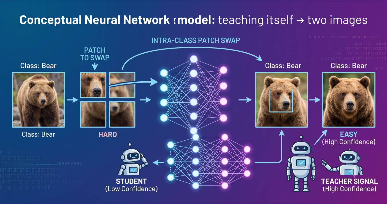
- The paper introduces intra-class patch swap, a data augmentation that trades small square patches between two images from the same class before feeding them into a single network.
- The swap creates a natural confidence gap, one image keeps the most recognizable parts and the other loses them, and the network is trained to match its own predictions across that gap.
- Unlike prior self-distillation methods, this approach needs no extra classifiers, no architectural changes, and no second network of any kind, just one augmentation function.
- Across image classification, semantic segmentation, and object detection, the method beats both existing self-distillation baselines and conventional teacher based distillation.
- On ImageNet with a ResNet50 backbone, the method even edges out training with a real, much larger ResNet152 teacher, using only one network.
The problem with needing a teacher at all
Knowledge distillation has been one of the most reliable tools for making a smaller, deployable model perform closer to a large, expensive one. The classic recipe trains a big teacher network first, then trains a compact student to mimic the teacher’s output distribution, not just the hard, one-hot labels. That extra signal, called soft knowledge, genuinely helps a smaller model converge to a better solution.
It also comes with real costs that rarely get discussed as prominently as the accuracy gains. Training a high capacity teacher before you can even start training your actual model doubles the compute budget and the storage footprint. Worse, there is no reliable rule for picking the right teacher for a given student, so practitioners are often left guessing, and the paper notes something genuinely counterintuitive from prior research, even a poorly trained teacher can still help a student, which only deepens the mystery of what is actually being transferred.
Self-distillation emerged as an answer to the teacher problem, letting one network act as its own teacher. But most existing self-distillation methods swap one cost for another. Methods like BYOT bolt extra classifier heads onto intermediate layers of the network, which complicates the architecture and makes the technique harder to transfer across different backbone types. Others rely on multi-stage training schedules or meta-learning routines that add their own computational overhead. The authors set out to build something that avoids both problems entirely, no extra network, no architectural surgery, and no complicated training schedule.
The core idea, teach yourself by comparing an easy view to a hard view
The method the authors land on is disarmingly simple to describe. Take two images from the same class. Divide each one into a grid of small square patches. Randomly select a subset of those patch positions and swap the patches at those positions between the two images. Feed both swapped images through the same single network, and train the network to make its predictions on one image agree with its predictions on the other, in addition to the ordinary cross entropy loss against the true label.
What makes this work is what the swap does to each image’s recognizability. If an animal’s head, the most visually distinctive part, happens to land entirely in one image after swapping, that image becomes an easy, high confidence example. The other image, left with only the body or tail, becomes a harder, lower confidence example. The network now has, for free, exactly the kind of confidence gap that a real teacher and student would normally have to be separately trained to produce.
Generating difficulty on purpose, not by accident
The authors are explicit that this difficulty gap is not guaranteed on every single swap, since the method does not use attention maps or any other mechanism to deliberately target the most discriminative region of an image. It relies on randomness. But because the swap happens fresh at every training iteration, the network is constantly presented with new easy and hard pairings rather than settling into one static difficulty level. Matching predictions across a bigger confidence gap produces a larger loss contribution, so the training process naturally weights its attention toward whichever image pairs show the sharpest difference in difficulty at any given step, discouraging the network from settling into a comfortable groove where only the easiest, most obvious examples drive learning.
Keeping the class relationships intact
The paper draws a sharp and well illustrated contrast with mix based augmentations like MixUp and CutMix, which blend two images from potentially unrelated classes together. The authors show a striking piece of evidence for why that matters, a histogram of a model’s predicted probabilities on a misclassified baby photo. A model trained with CutMix assigns meaningful probability to categories like clock, flatfish, and pear, categories with no semantic relationship to a baby at all, because CutMix literally pasted parts of unrelated images into the training data. A model trained with intra-class patch swap, by contrast, distributes its uncertainty across boy, girl, man, and woman, categories that are actually related to the target class. Because the swap only ever happens between two images that already share the same label, the underlying object’s identity, and its relationship to visually similar classes, is never corrupted the way it can be with cross-class mixing.
The actual training objective
Underneath the intuition sits a fairly compact loss function. Both swapped images still get trained against their shared true label using ordinary cross entropy, since learning the hard label correctly is still the primary task. On top of that, the network’s softened output distributions for the two swapped images are pulled toward each other using a symmetric KL divergence, computed both directions between the pair, with a temperature parameter that smooths the probability distribution before comparison. The two loss terms, cross entropy and the distillation term, are combined with equal weighting in the paper’s main experiments.
One deliberate design choice stands out against a closely related prior method called CS-KD, which performs a similar kind of same-class consistency matching but detaches the gradient on one of the two samples, effectively treating it as a fixed, offline teacher. This paper’s authors backpropagate through both swapped images fully, on the reasoning that a detached sample cannot reliably provide the same quality of supervision a genuine pretrained teacher would, so cutting the gradient there throws away signal the network could otherwise use.
Why the authors think this actually improves training, not just accuracy
Beyond the headline accuracy numbers, the paper digs into a few concrete, testable explanations for why the swap helps, rather than treating the improvement as a black box.
It appears to fight vanishing gradients
The authors measure the average magnitude of gradients flowing through each convolutional layer of a ResNet18 trained on CIFAR100, with and without the patch swap. Without the swap, gradient magnitudes in several layers stay very small throughout training, meaning those layers are barely being updated and are effectively going to waste. With the swap enabled, gradient magnitudes rise noticeably across the same layers, suggesting the harder, swapped examples are forcing more of the network’s capacity to stay actively engaged during training rather than sitting idle.
It keeps generating challenge throughout training rather than tapering off
A second experiment tracks the L1 norm of the distillation loss’s gradient over the full course of training. Without patch swap, this gradient signal drops sharply after roughly one hundred fifty epochs and stays low, a pattern consistent with the network having converged early and settled into a comfortable, low challenge regime. With patch swap enabled, the gradient signal stays meaningfully higher for the remainder of training, which the authors interpret as evidence the model keeps learning throughout, rather than plateauing early on the easiest examples.
It narrows the gap between training and testing accuracy
Because the method pairs up two images per training step, it effectively doubles the input batch at each iteration, an effect the authors compare to prior research on large batch training, which found that larger, less noisy gradient estimates tend to bias optimization toward sharp minima that generalize less well. Consistent with that concern, a network trained on doubled batches without the patch swap shows a very high training accuracy but a comparatively larger gap down to test accuracy. Adding the patch swap narrows that gap substantially across every architecture the authors test, from ninety nine percent training accuracy without swap for a ResNet18, for example, down to a lower but far more test consistent ninety eight and a half percent training accuracy with the swap, alongside a genuinely higher test accuracy.
How well does it actually perform
The results span three distinct computer vision tasks, and the pattern holds up across all of them.
Image classification
On ImageNet with a ResNet50 backbone, the method improves top-1 accuracy by one and a half percentage points over plain hard label training, and notably outperforms every other self-distillation baseline tested, including BYOT, TF-KD, and CS-KD. The comparison that stands out most is against genuine teacher based distillation, training the same ResNet50 student against a real, much larger ResNet152 teacher using classic knowledge distillation actually underperforms this teacher free method, despite the ResNet152 teacher itself having no student to answer to. The authors also confirm the method generalizes across very different network families, testing it on the lightweight MobileNetV2 and on MViTv2, a transformer based architecture, and finding meaningful gains in both cases, evidence the technique is not tied to convolutional architectures specifically.
On CIFAR100, across eight different backbone architectures ranging from ResNet18 up through ResNet101, VGG13, VGG16, and both ShuffleNet variants, the method posts the best top-1 accuracy in every single case among a field of nine competing self-distillation baselines, with improvements over plain hard label training ranging from roughly two and a half to nearly three and a half percentage points depending on the architecture. On fine grained datasets, where the task specifically requires distinguishing subtle differences between visually similar subcategories, the gains grow even larger, up to a twelve point improvement on the CUB-200-2011 bird dataset with a ResNet18 backbone.
| Method | ResNet18 | ResNet50 | VGG16 | ImageNet, ResNet50 top-1 |
|---|---|---|---|---|
| Hard label baseline | 77.92% | 79.01% | 74.40% | 76.30% |
| BYOT | – | – | – | 76.96% |
| CS-KD | 78.85% | 78.99% | 74.92% | 76.78% |
| DLB | 80.25% | 81.35% | 76.58% | – |
| Teacher based KD, ResNet152 teacher | – | – | – | 77.49% |
| Intra-class patch swap (ours) | 80.53% | 81.97% | 77.66% | 77.85% |
Semantic segmentation and object detection
To test whether a backbone pretrained with this method actually transfers useful features to other tasks, the authors take a ResNet50 distilled on ImageNet and drop it into a DeepLabV3+ segmentation network, evaluating on Pascal VOC2012 and Cityscapes. Mean intersection over union improves by nearly three points on VOC2012 and just over two points on Cityscapes compared to the same backbone trained with plain hard labels. On the more demanding RUGD dataset, which segments unstructured off road terrain into coarse categories like smooth regions, rough regions, and obstacles, the method reaches the best reported mean intersection over union among a wide field of specialized segmentation architectures, including several transformer based methods, improving over the hard label baseline by roughly four points overall and by a striking twenty two points specifically on the smooth region category.
On object detection, using a Single Shot Detector with the same distilled ResNet50 backbone on Pascal VOC, the method outperforms the hard label baseline on fourteen out of twenty object categories and improves mean average precision from 76.13 to 77.29.
Does it hold up under stress, noisy labels and adversarial attacks
A method that only wins on clean benchmark accuracy is a weaker result than one that also improves robustness, and the authors test both directly. Under label noise, where a fraction of training labels are deliberately flipped to incorrect values, the method consistently posts the highest test accuracy across every noise level tested, including a meaningful gap over both plain hard label training and label smoothing at an aggressive eighty percent noise rate. Under white box adversarial attacks using FGSM and its iterative variant, the gap widens further as the attack strength increases, at the largest perturbation tested the method retains over twenty percent accuracy where every other baseline collapses to under five percent. The authors also report improved calibration metrics, meaning the model’s confidence scores better reflect its actual accuracy, and improved robustness to common image corruptions like blur, fog, and contrast shifts, though the calibration and corruption gains are comparatively more modest than the classification and adversarial results.
Getting the patch size and swap rate right
Two hyperparameters matter most in practice, the size of the patches being swapped and the probability that a given pair of images gets swapped at all. Across a broad sweep, a swap probability of point five generally produces the best results compared to no swapping at all, and dividing images into a four by four grid of patches generally outperforms a coarser two by two grid, suggesting that finer, more localized patch exchange helps the network learn from smaller, more partial pieces of visual evidence rather than large, blunt regions. The authors also find that gradually ramping the swap probability up over the course of training, starting low and increasing toward point five as training progresses, outperforms holding the probability fixed throughout, a pattern they connect to curriculum learning, letting the network first stabilize on clean, unperturbed features before gradually introducing harder, swapped examples.
Honest limitations worth keeping in mind
The authors are candid that the difficulty gap this method depends on is not guaranteed on any individual swap, since the technique relies on randomness rather than deliberately targeting an image’s most discriminative region, and they frame this as a conscious tradeoff of precise control for simplicity and broad applicability rather than an oversight. They also report that the swap augmentation alone, without the self-distillation loss, produces essentially no benefit on its own, meaning the gains come specifically from the combination of the augmentation and the distillation objective together, not from either piece in isolation. The method also doubles the effective batch size at every training step, which the authors note mirrors known large batch training tradeoffs and required them to tune the swap probability carefully rather than assume any setting would work. Finally, while the calibration and corruption robustness results are generally favorable, they are less consistently dominant than the classification and adversarial results, with some individual corruption types and calibration metrics where competing augmentations like MixUp or CutOut hold a narrow edge.
Conclusion
The central achievement here is showing that a genuinely useful teacher signal does not require a second network at all, just a clever way of generating two different views of the same underlying content and asking a single model to reconcile its own confidence between them. Swapping patches between same-class images produces exactly the kind of asymmetry, one confident view and one uncertain view, that conventional distillation normally has to train an entire separate teacher network to produce.
The more interesting conceptual point is what this implies about where distillation’s real value has been coming from all along. If a single network with no external teacher can match or beat training against a genuine, much larger pretrained teacher, as it does here against a ResNet152, that is a meaningful data point suggesting the benefit of distillation may have less to do with the teacher’s absolute capability and more to do with the structure of the training signal itself, a well shaped confidence gap paired with preserved class relationships.
Whether this finding generalizes to domains further from natural image benchmarks, language models, audio, or tabular data, is an open question the paper does not attempt to answer, and the patch based mechanism specifically depends on spatial structure that not every data modality shares.
The remaining gaps, an inherently random rather than guaranteed difficulty gap, a doubled effective batch size that demands careful tuning, and modestly mixed results on calibration and corruption robustness, all mark reasonable directions for follow up work rather than undermining the central result. The authors themselves point toward automating the hyperparameter search and exploring combinations of intra-class and inter-class augmentation as next steps.
What is worth carrying away from this paper is the reminder that a lot of what makes knowledge distillation work might be simpler and more mechanical than the teacher-student framing suggests. Sometimes the most useful teacher a model can have is just a slightly easier version of the same picture it is already looking at.
A runnable implementation of intra-class patch swap and the self-distillation loss
The following is an independent, simplified but complete and runnable reimplementation of the paper’s augmentation and training objective, including the patch swap function, the combined cross entropy and KL divergence loss, a training loop, and a smoke test on synthetic data.
import torch.nn as nn
import torch.nn.functional as F
# —————————————————————–
# Intra-class patch swap augmentation, following Section 3.2
# Divides each image into a grid of patches and randomly exchanges a
# subset of them between two same-class images in the batch
# —————————————————————–
def intra_class_patch_swap(images_a, images_b, patch_size, swap_prob=0.5):
“””images_a, images_b, shape (batch, channels, height, width), each pair
(images_a[i], images_b[i]) must share the same class label. Returns the
two swapped tensors, same shape as the inputs.”””
batch, channels, height, width = images_a.shape
grid_h, grid_w = height // patch_size, width // patch_size
total_patches = grid_h * grid_w
# unfold into non overlapping patches, shape (batch, channels * patch_size**2, total_patches)
patches_a = F.unfold(images_a, kernel_size=patch_size, stride=patch_size)
patches_b = F.unfold(images_b, kernel_size=patch_size, stride=patch_size)
swapped_a = patches_a.clone()
swapped_b = patches_b.clone()
for i in range(batch):
if torch.rand(1).item() >= swap_prob:
continue # this pair stays unswapped
# pick a random, non empty, non total subset of patch positions to exchange
num_to_swap = torch.randint(1, total_patches, (1,)).item()
swap_positions = torch.randperm(total_patches)[:num_to_swap]
temp = swapped_a[i, :, swap_positions].clone()
swapped_a[i, :, swap_positions] = swapped_b[i, :, swap_positions]
swapped_b[i, :, swap_positions] = temp
# fold back into images
images_a_hat = F.fold(swapped_a, output_size=(height, width), kernel_size=patch_size, stride=patch_size)
images_b_hat = F.fold(swapped_b, output_size=(height, width), kernel_size=patch_size, stride=patch_size)
return images_a_hat, images_b_hat
# —————————————————————–
# Combined loss, cross entropy on hard labels plus a symmetric KL
# divergence between the two swapped predictions, following Eq. 1 to Eq. 3
# —————————————————————–
def self_distillation_loss(logits_a, logits_b, labels, temperature=4.0, gamma=1.0, alpha=1.0):
ce_a = F.cross_entropy(logits_a, labels)
ce_b = F.cross_entropy(logits_b, labels)
log_probs_a = F.log_softmax(logits_a / temperature, dim=1)
log_probs_b = F.log_softmax(logits_b / temperature, dim=1)
probs_a = log_probs_a.exp()
probs_b = log_probs_b.exp()
# KL(a, b) and KL(b, a), each scaled by temperature squared as in the paper
kd_ab = (temperature ** 2) * F.kl_div(log_probs_b, probs_a, reduction=“batchmean”)
kd_ba = (temperature ** 2) * F.kl_div(log_probs_a, probs_b, reduction=“batchmean”)
total_loss = 0.5 * gamma * (ce_a + ce_b) + 0.5 * alpha * (kd_ab + kd_ba)
return total_loss
# —————————————————————–
# Minimal training step, following Algorithm 1
# —————————————————————–
def training_step(model, optimizer, images_a, images_b, labels, patch_size, swap_prob):
swapped_a, swapped_b = intra_class_patch_swap(images_a, images_b, patch_size, swap_prob)
optimizer.zero_grad()
logits_a = model(swapped_a)
logits_b = model(swapped_b)
loss = self_distillation_loss(logits_a, logits_b, labels)
loss.backward()
optimizer.step()
return loss.item()
# —————————————————————–
# Smoke test, a tiny CNN trained for a few steps on synthetic same-class
# image pairs to confirm the augmentation and loss run end to end
# —————————————————————–
def run_smoke_test():
torch.manual_seed(0)
num_classes, batch, image_size, patch_size = 10, 16, 32, 8
model = nn.Sequential(
nn.Conv2d(3, 16, 3, padding=1), nn.ReLU(), nn.AdaptiveAvgPool2d(1),
nn.Flatten(), nn.Linear(16, num_classes),
)
optimizer = torch.optim.SGD(model.parameters(), lr=0.05)
for step in range(20):
labels = torch.randint(0, num_classes, (batch,))
# two independently sampled, same-class image tensors per pair,
# standing in for two real photos of objects from the same class
images_a = torch.randn(batch, 3, image_size, image_size)
images_b = torch.randn(batch, 3, image_size, image_size)
loss_value = training_step(model, optimizer, images_a, images_b, labels, patch_size, swap_prob=0.5)
if step % 5 == 0:
print(f”step {step}, loss {loss_value:.4f}”)
if __name__ == “__main__”:
run_smoke_test()
Running this trains a tiny convolutional network for twenty steps on random same-class image pairs, applying the patch swap and the combined loss at every step, and prints the loss so you can confirm the whole pipeline, the swap, the forward pass on both swapped images, and the joint cross entropy plus KL divergence objective, runs correctly end to end before swapping in a real backbone and a real dataset.
Go straight to the source
This article summarizes and analyzes the original research. Read the full methodology, every result table across classification, segmentation, and detection, and the complete ablation studies directly from the preprint, and check the authors’ own repository for their reference implementation.
Read the paper View the code repositoryFrequently asked questions
What is self-distillation and how is it different from regular knowledge distillation?
Regular knowledge distillation trains a smaller student network to mimic a separate, pretrained teacher network. Self-distillation instead trains a single network to act as its own teacher and student at once, without ever needing a second model.
What exactly does intra-class patch swap do?
It divides two images from the same class into a grid of small square patches, randomly exchanges a subset of those patches between the two images, and trains the network to match its predictions across the resulting pair, which naturally differ in how easy they are to classify.
Why does swapping patches between same-class images work better than mixing different classes?
Because the swap never changes which class an image belongs to, the model’s understanding of how that class relates to visually similar classes stays intact. Methods that blend unrelated classes together, like CutMix, can teach the model to associate a class with semantically unrelated categories.
Does this method require any changes to the network’s architecture?
No. It works with any existing backbone unchanged, requiring only the patch swap augmentation function and the distillation loss added to training, which is why the authors were able to test it on convolutional networks like ResNet and VGG as well as a transformer based architecture without modification.
How much does patch size matter?
It matters measurably. In the paper’s sweep, a finer four by four patch grid generally outperformed a coarser two by two grid, and a swap probability around one half generally produced the best results compared to no swapping at all.
Does this replace the need for a teacher network entirely?
In the settings tested here, largely yes. The paper reports that training a ResNet50 with this method outperforms training the same ResNet50 against a real, much larger ResNet152 teacher using conventional distillation.
Academic citation. Choi, H., Jeon, E. S., Shukla, A., and Turaga, P. Intra-class patch swap for self-distillation. Preprint submitted to Neurocomputing, arXiv:2505.14124, 2025.
This analysis is based on the published preprint and an independent evaluation of its claims.
Pingback: 7 Shocking Truths About Trace-Based Knowledge Distillation That Can Hurt AI Trust - aitrendblend.com