
Key points
- Researchers from Saudi Arabia, Ecuador, Kyrgyzstan, the United Arab Emirates, and Egypt built a four stage pipeline called DMBOTL-MRDD to classify fundus photographs into seven categories including diabetic retinopathy, glaucoma, and age related macular degeneration.
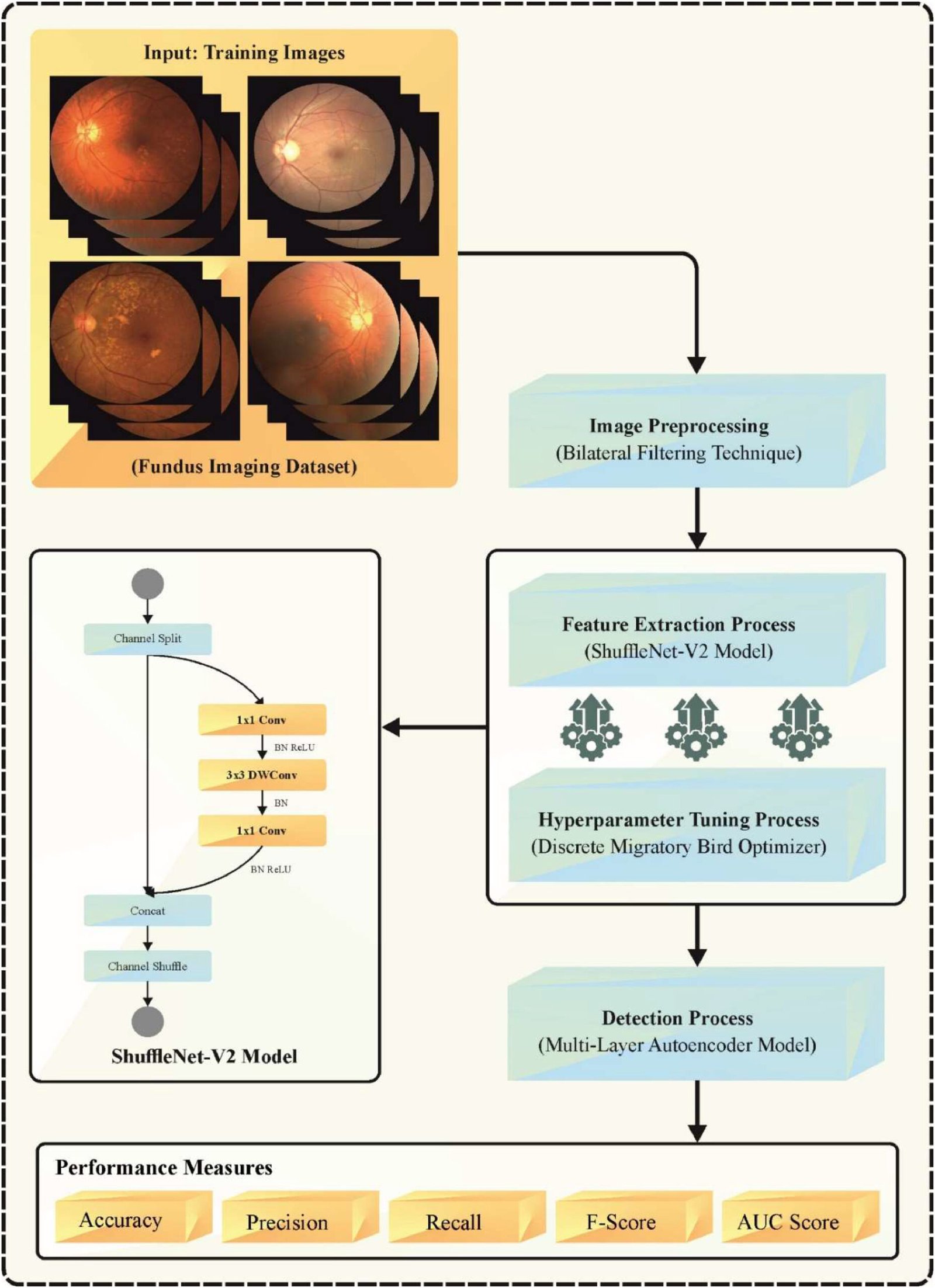
- The pipeline denoises images with a Wiener filter, pulls features with the lightweight ShuffleNetv2 network, tunes that network’s settings with a Discrete Migratory Bird Optimizer, and classifies the result with a multilayer autoencoder.
- On a benchmark set of 1292 fundus images the method reported an average accuracy of 97.12 percent, ahead of seven comparison methods the authors tested against, including a prior autoencoder based approach called IDL-MRDD at 96.31 percent.
- Precision and recall trailed accuracy noticeably, landing near 90 percent and 89 percent, which matters more than the headline accuracy number for a screening tool.
- The dataset itself is small by deep learning standards and one class, labeled HR, contains only 92 images against 200 for every other class, a detail the authors acknowledge as a limitation.
- This is a laboratory benchmark result from a peer reviewed journal article, not a validated clinical device, and nothing here should be read as diagnostic guidance.
The problem this pipeline is actually trying to solve
Retinal disease does not announce itself early. Age related macular degeneration, diabetic retinopathy, and glaucoma can all progress for years before a patient notices anything wrong, and by the time vision loss is obvious a meaningful amount of it can already be permanent. The paper’s authors, led by Nouf Al Kahtani at Imam Abdulrahman bin Faisal University with coauthors at Universidad Tecnológica Indoamérica in Ecuador, the University of Central Asia, Ajman University, and South Valley University in Egypt, frame the challenge in fairly plain terms. Fundus photography is cheap and fast. The rods and cones that do the actual seeing, roughly one hundred million rods and six to eight million cones by the estimate the paper cites, generate a lot of visual information that a specialist has to interpret one image at a time.
That interpretation bottleneck is not a new observation. What is worth paying attention to here is how narrowly most automated systems have tried to address it. A model trained only to flag diabetic retinopathy will say nothing useful about a glaucoma case sitting in the same batch of images. A model trained on hand picked features chosen by an engineer will drift the moment those features stop matching a new population of patients. The paper’s stated goal is to build something that looks at one photograph and sorts it across several possible conditions at once, which is a meaningfully harder task than the binary yes or no screening that dominates a lot of prior work in this space.
What came before it
The related work section of the paper is a useful map of how crowded this subfield already is. Aslam and colleagues built a six layer convolutional network trained on data pooled from three sources to classify twenty different retina related conditions. Vaiyapuri and coauthors, whose method the current paper uses as its main point of comparison under the label IDL-MRDD, combined a metaheuristic threshold segmentation step with a SqueezeNet feature extractor and a stacked sparse autoencoder classifier. Belharar and Zrira built something called DeepRetino aimed at six retinal illnesses using CLAHE contrast enhancement ahead of a CNN. Bashir and colleagues proposed RDS-DR, mixing residual and dense blocks specifically for diabetic retinopathy severity grading, while Sajid and colleagues took a similar severity grading problem and built DR-NASNet around an improved NASNet backbone.
None of that is small work, and the current paper does not pretend otherwise. Its authors summarize the field’s shared weaknesses plainly. Models trained with heavy preprocessing or specific augmentation strategies tend to struggle on lower quality images from a different clinic or camera. Approaches built around metaheuristic search or contrast enhancement can be computationally expensive to run. Transfer learning based systems and residual dense networks often generalize poorly to rare conditions or to patient populations that look different from the training set. The gap the authors are trying to fill, in their own framing, is a system that holds up across varying image quality, noise levels, and patient populations, while still running efficiently enough to be practical.
You can read a healthy amount of skepticism into that framing. Every paper in this genre claims to fill exactly the gap its predecessors left open. What sets this one apart is not the claim, it is the specific set of engineering choices made to chase it, particularly the decision to reach for a hyperparameter search algorithm modeled on how migratory birds travel in a V formation.
How the DMBOTL-MRDD pipeline actually works
The system name is a mouthful. DMBOTL-MRDD stands for Discrete Migratory Bird Optimizer with Transfer Learning aided Multi Retinal Disease Detection, and it breaks cleanly into four stages that run one after another on each fundus photograph.
Stage one, cleaning up the image with a Wiener filter
Fundus cameras, like any imaging device, introduce noise, and that noise can hide the fine vascular detail a diagnosis depends on. The paper’s first stage applies Wiener filtering, a classical signal processing technique that estimates local mean and variance across the image and adapts its smoothing accordingly rather than blurring everything uniformly the way a plain Gaussian blur would. The authors argue this preserves edges better, which matters a great deal in fundus photography since the optic disc boundary, the blood vessel branching pattern, and small hemorrhages or drusen deposits are exactly the features later stages need to see clearly. It is a fairly standard preprocessing choice, not the paper’s novel contribution, but it is a sensible one given what the rest of the pipeline is trying to extract.
Stage two, feature extraction with ShuffleNetv2
Once the image is denoised, the paper hands it to ShuffleNetv2, a convolutional network originally designed for mobile and edge deployment. ShuffleNetv2 gets its efficiency from two tricks working together, channel splitting combined with pointwise and depthwise convolutions, and a channel shuffle operation that lets information mix across the split groups without the heavy computational cost of a full convolution. The appeal for a project like this one is straightforward. A model this size can run on far less hardware than something like ResNet or VGG while still learning a useful feature representation, which matters if the eventual goal is deployment in a clinic that does not have a server room full of GPUs.
Worth noting, the paper’s own description of why it chose ShuffleNetv2 briefly references a completely different use case, a plant disease dataset with forty one classes, before returning to the retinal task. That looks like a drafting artifact carried over from the architecture’s original justification in prior literature rather than a claim specific to this dataset, and it is the kind of small inconsistency worth flagging rather than smoothing over.
Stage three, tuning the network with a Discrete Migratory Bird Optimizer
This is the paper’s actual novelty, and it deserves the most attention. Any convolutional network like ShuffleNetv2 has a set of hyperparameters, things like pooling configuration, the number of shuffle units, the scale factor, and the bottleneck percentage, that need to be set correctly for the network to perform well. Grid search tries every combination and is slow. Random search is faster but blind. The authors instead borrow an idea from how migratory birds actually fly, forming their whole population into a V shape with one leader bird cutting through the air first and the rest trailing behind on two diagonal lines.
In the algorithm’s version of that flight, each of the n candidate hyperparameter configurations plays the role of one bird. A stronger candidate gets picked as the leader, and the rest split into left and right lines. On each generation, the leader searches its own neighborhood for better solutions using mutation and crossover operators, while the follower birds do the same and compare their results against whichever neighbor bird is ahead of them. Unused good solutions found by the leader get passed back to help the followers improve, roughly mirroring how a bird drafting behind another in real flight benefits from the lead bird’s effort. Three separate mutation strategies, covering task sequence changes, position changes, and workplace reassignment, keep the search from collapsing into a single local optimum too early. The whole process runs until a fixed number of iterations completes, and it selects the configuration that maximizes a precision based fitness score.
The reason this approach is attractive for hyperparameter tuning specifically is that many of the choices involved, like the number of shuffle units or a pooling strategy, are categorical rather than continuous. Gradient based tuning approaches do not have a clean way to handle that kind of discrete decision, while a population based search like this one does, since it just compares whole candidate solutions to each other rather than trying to differentiate through them.
Why the bird metaphor matters more than it sounds
It would be easy to read Discrete Migratory Bird Optimizer as a marketing flourish borrowed from nature inspired computing, and to some extent that whole subfield does lean on catchy names. But the actual mechanism, a leader sharing discovered solutions with followers arranged in a V, maps onto a real advantage over blind random search, namely that good partial solutions get reused instead of discarded, and the search space narrows over successive generations rather than staying uniformly wide. That is the part worth remembering after the bird imagery fades.
Stage four, classification with a multilayer autoencoder
The last stage takes the tuned feature vectors and runs them through a multilayer autoencoder, a network built from an encoder that compresses the input into a smaller latent representation and a decoder that tries to reconstruct the original from that compressed form. Autoencoders are typically framed as unsupervised tools since they learn to compress and reconstruct data without needing labeled examples, and the authors lean on that property, arguing it makes the system less dependent on large labeled datasets, which matters in a medical imaging context where labeled data is expensive to produce and rare disease categories are, by definition, rare.
The encoder and decoder in this design are built from fully connected layers rather than convolutions at this stage, since the convolutional feature extraction already happened back in stage two. The math the paper lays out for a fully connected layer is standard, mapping an input vector through a weight matrix and a bias term before an activation function, and the network is trained to minimize the squared difference between its output and its input across the whole layer.
\( \text{Loss} = \dfrac{1}{H}\sum_{i=0}^{H-1}(x_i – z_i)^2 \)
Here \(x\) is the input to a given fully connected layer and \(y\) is its output, \(W\) is the learned weight matrix, \(b\) is the bias term, and \(\delta\) is the activation function. In the loss equation, \(x_i\) and \(z_i\) are the input and reconstructed output of the \(i\) th neuron and \(H\) is the total number of input neurons. That reconstruction objective is what actually drives the model to learn a compact representation of what a healthy retina versus a diseased one looks like in the latent space, which the classifier head then uses to make its seven way decision.
How the weights actually get updated
Training the ShuffleNetv2 backbone end to end, meaning without freezing any layers, uses the Adam optimizer, and the paper walks through the standard Adam update rule in full. It is worth including here because it is the same optimizer doing the heavy lifting in a large share of modern computer vision work, retinal imaging or otherwise.
\( \rho_m \leftarrow \beta_m \rho_m \)
\( \rho_v \leftarrow \beta_v \rho_v \)
\( m \leftarrow \beta_m m + (1-\beta_m)\nabla_w J \)
\( v \leftarrow \beta_v v + (1-\beta_v)(\nabla_w J \odot \nabla_w J) \)
\( w \leftarrow w – \alpha \left( \dfrac{m}{\sqrt{v}+\epsilon} \dfrac{\sqrt{1-\rho_v}}{1-\rho_m} \right) \)
The terms \(m\) and \(v\) track the first and second moment estimates of the gradient, \(\beta_m\) and \(\beta_v\) are the exponential decay rates controlling how much weight recent gradients get, \(\rho_m\) and \(\rho_v\) handle the bias correction that keeps early training steps from being skewed toward zero, \(\alpha\) is the learning rate, and \(\epsilon\) is a small constant included purely to stop the update from dividing by zero. None of this is specific to retinal imaging, it is textbook Adam, and the paper is honest that it is using the standard formulation rather than a modified one.
How the bird optimizer scores a candidate solution
The fitness function the migratory bird search optimizes against is deliberately simple, precision on the classification task.
\( P = \dfrac{TP}{TP + FP} \)
where \(TP\) is true positives and \(FP\) is false positives for a given candidate configuration. Choosing precision alone as the fitness signal is a defensible engineering shortcut, since it is cheap to compute during search and it directly rewards configurations that avoid false alarms. It is also a choice with a real tradeoff attached, because optimizing for precision alone can quietly favor configurations that are more conservative about calling something diseased, at some cost to recall, and recall is arguably the more clinically important number in a screening context where missing a real case is worse than flagging a healthy one for a second look. The results section bears that tradeoff out, which the next section covers directly.
What the numbers actually show
The authors tested their pipeline on a benchmark fundus imaging dataset of 1292 images spanning seven classes, image sizes running either 1444 by 1444 or 2304 by 1728 pixels. The class breakdown is AMD, DR meaning diabetic retinopathy, Glaucoma, a class labeled HR, Normal, an Others category, and Pathological Myopia, with 200 images in every class except HR, which has only 92.
| Class | Images |
|---|---|
| AMD | 200 |
| DR | 200 |
| Glaucoma | 200 |
| HR | 92 |
| Normal | 200 |
| Others | 200 |
| Pathological Myopia | 200 |
| Total | 1292 |
The paper does not spell out in its main text what HR stands for. In other fundus imaging datasets that use the same abbreviation it typically refers to hypertensive retinopathy, but since this paper itself never defines the term explicitly, that reading should be treated as likely context rather than a claim the authors made directly.
Across a 80 percent train and 20 percent test split, the model’s average accuracy came in at 97.12 percent on the training partition and 97.02 percent on the held out test partition, with average precision around 90 percent, average recall around 89 percent, an F1 score near 89.4 percent, and a Matthews correlation coefficient near 87.8 percent. A second run using a 70 percent train and 30 percent test split produced very similar numbers, 97.03 percent training accuracy and 96.61 percent test accuracy.
The gap between accuracy in the high nineties and precision or recall in the high eighties is the single most important thing to sit with in this whole results section. Accuracy on a seven class dataset like this one gets inflated by every correct call across every class, including the easy ones, while precision and recall are more sensitive to the specific mistakes that matter clinically, false positives that send a healthy patient for unnecessary follow up and false negatives that miss a real disease. A 97 percent headline number reads as close to solved. An 89 percent recall means roughly one in nine positive cases across the dataset would be missed on average, and that number varies meaningfully by class, dropping to about 79 percent recall for diabetic retinopathy on the smaller test split and about 81 percent recall for the HR class in the 80 percent training run, exactly the class with the fewest training examples.
| Class | Accuracy | Precision | Recall | F1 score |
|---|---|---|---|---|
| AMD | 97.39 | 94.81 | 88.48 | 91.54 |
| DR | 96.61 | 90.85 | 85.43 | 88.05 |
| Glaucoma | 98.45 | 92.94 | 97.53 | 95.18 |
| HR | 97.97 | 90.16 | 78.57 | 83.97 |
| Normal | 97.48 | 91.12 | 93.33 | 92.22 |
| Others | 96.13 | 86.59 | 88.75 | 87.65 |
| Pathological Myopia | 95.84 | 83.82 | 90.62 | 87.09 |
Per class results on the 80 percent training partition, all values in percent, from Table 2 of the source paper.
That pattern lines up neatly with the precision focused fitness function the bird optimizer was searching against. A search that rewards precision without an equal weight on recall will tend to produce a model that is good at not crying wolf and somewhat worse at catching every real case, and the class level numbers above are consistent with exactly that outcome, most visibly on the HR class, which is both the hardest class in the recall numbers and the class with the least training data by a wide margin.
How it stacks up against other methods
The paper compares its full pipeline against seven other approaches, all evaluated on accuracy, precision, recall, and F1 score.
| Method | Accuracy | Precision | Recall | F1 score |
|---|---|---|---|---|
| DMBOTL-MRDD | 97.12 | 90.04 | 88.96 | 89.39 |
| IDL-MRDD | 96.31 | 87.31 | 87.81 | 86.21 |
| RBF | 83.11 | 83.91 | 83.01 | 83.21 |
| MLP | 81.51 | 82.11 | 81.31 | 81.81 |
| SVM | 81.51 | 82.11 | 81.41 | 81.71 |
| CNN-DL | 80.91 | 81.21 | 80.51 | 81.01 |
| ANN | 75.01 | 75.91 | 74.91 | 75.11 |
| NB | 66.91 | 67.21 | 78.31 | 74.71 |
From Table 3 of the source paper, comparing against Vaiyapuri and colleagues’ IDL-MRDD method and six classical or general purpose classifiers.
The gap between DMBOTL-MRDD and IDL-MRDD, its closest competitor, is under one percentage point on accuracy. The gap between both of those methods and everything else on the list, a set of more generic classifiers including a plain CNN, a multilayer perceptron, a radial basis function network, a support vector machine, a basic artificial neural network, and naive Bayes, is enormous, ranging from fourteen to thirty points. That contrast says less about how special the bird optimizer specifically is and more about how much a purpose built pipeline with proper preprocessing and transfer learning outperforms a generic off the shelf classifier on this kind of image task, which is a well established pattern in medical imaging research generally, not something unique to this paper.
The headline accuracy number is doing a lot of the persuasive work here, and it is precision and recall, quietly sitting in the high eighties, that tell the more honest story. Editorial analysis, aitrendblend
The clinical translation gap
There is real distance between a 97.12 percent accuracy figure reported in a paper and a system a hospital could actually rely on, and it is worth walking through where that distance comes from rather than treating the two as interchangeable.
First, the dataset. 1292 images across seven classes is workable for demonstrating that a pipeline functions, but it is small relative to the population diversity a real screening deployment would face, different cameras, different lighting conditions, different ethnic populations with different baseline retinal pigmentation, and different comorbidities layered on top of the primary disease being screened for. The paper’s own conclusion acknowledges this directly, naming dataset size as a real constraint on how well the model would generalize to a broader population.
Second, the class imbalance in the HR category, at 92 images against 200 for every other class, is exactly the kind of imbalance that tends to produce a model which is quietly worse at the underrepresented class than the aggregate numbers suggest, and the recall figures for HR bear that out, sitting noticeably lower than most other classes across both train and test splits.
Third, this is a single benchmark dataset evaluated with a single train and test split methodology repeated at two different ratios. There is no external validation set from a different hospital, clinic, or country reported in the paper, which is the step that would actually demonstrate the model holds up outside the exact data distribution it was tuned on. That absence is not a flaw unique to this paper, it is close to the norm for early stage academic work in this space, but it is precisely the gap that separates a promising benchmark result from a tool ready for clinical use.
Fourth, nothing in the paper describes regulatory clearance, prospective clinical trial results, or deployment in an actual care setting. The work sits at the research and development stage of the pipeline, which is a legitimate and useful stage of the process, but it is worth naming plainly rather than letting a strong accuracy number imply more than the study actually claims.
Honest limitations
The authors are reasonably direct about their own study’s weak points, and it is worth taking them at their word rather than glossing over the caveats section the way summaries of papers sometimes do.
- Sample size. 1292 total images is small for a deep learning pipeline with this many moving parts, and the authors state outright that this limits how confidently the model’s performance would generalize to a broader patient population.
- Class imbalance. The HR class has under half the images of every other category, and the paper notes generally that the study needs help dealing with imbalanced data, which risks biased predictions for underrepresented disease categories, a pattern that shows up concretely in the lower recall scores for that class.
- Image quality sensitivity. The authors flag that discrepancies in image quality or noise could influence performance, particularly on real world fundus images that may look nothing like the relatively clean benchmark set used here.
- Real time readiness. Despite choosing a lightweight backbone specifically for efficiency, the authors note their own method would need additional optimization for real time clinical application, meaning the current results describe offline benchmark performance rather than a live clinic workflow.
- Single dataset, single methodology. All reported numbers come from one dataset evaluated with train and test splits rather than an independent external validation cohort, which the paper does not report having access to.
None of these limitations undercut the paper’s core engineering contribution, which is a working demonstration that a bird flight inspired search algorithm can meaningfully improve hyperparameter selection for a lightweight CNN on this kind of task. They do mean the 97.12 percent number should be read as a solid benchmark result rather than a finished clinical product, and the paper itself, to its credit, does not claim otherwise in its conclusion.
Where this fits in the bigger picture
Step back from the specific architecture and the more durable idea here is about search strategy rather than any single network choice. Convolutional networks like ShuffleNetv2 have a lot of hyperparameters that interact with each other in ways that are hard to reason about by hand, and nature inspired population search algorithms, whether modeled on bird migration, ant foraging, or particle swarms, keep showing up across medical imaging papers as a practical middle ground between exhaustive grid search and blind random search. What differs from paper to paper is mostly the specific mutation and crossover strategy and the fitness function chosen to guide the search, and this paper’s choice of precision as that fitness signal is a design decision with visible consequences in its own results, not a neutral default.
For an engineer building a similar pipeline for a different medical imaging task entirely, whether that is skin lesion classification, chest X-ray triage, or histopathology slide scoring, the transferable lesson is less about retinal disease specifically and more about the general pattern, pair a lightweight efficient backbone with a discrete population based hyperparameter search when your hyperparameters are categorical, and be deliberate about what your fitness function optimizes for, since it will shape your precision recall tradeoff whether you intend it to or not.
The one number worth remembering
Not 97.12 percent. The number worth carrying forward is the roughly seven to eight point gap between accuracy and recall across most classes, and the wider gap on the smallest class. That gap is where the real clinical risk of a system like this one lives, and it is the number any future version of this work should try to close first.
A worked implementation sketch
The code below is an independent, simplified reimplementation written for this article to illustrate the pipeline’s structure. It uses a small ShuffleNetv2 style feature extractor, a compact stand in for the discrete bird optimizer search over a categorical hyperparameter space, and a multilayer autoencoder classifier head trained with a reconstruction loss plus a classification loss, run end to end on random dummy data as a smoke test. It is meant for readers who want to see the architecture take concrete shape in code, not as a copy of the authors’ own implementation, which was not published alongside the paper.
# Independent PyTorch sketch of a DMBOTL-MRDD style pipeline
# Wiener style denoise -> ShuffleNetv2 style features -> discrete bird search -> multilayer autoencoder classifier
import torch
import torch.nn as nn
import torch.nn.functional as F
import random

class ShuffleUnit(nn.Module):
    # One ShuffleNetv2 style block, channel split, depthwise conv, channel shuffle
    def __init__(self, channels):
        super().__init__()
        half = channels // 2
        self.branch = nn.Sequential(
            nn.Conv2d(half, half, 1, bias=False),
            nn.BatchNorm2d(half),
            nn.ReLU(inplace=True),
            nn.Conv2d(half, half, 3, padding=1, groups=half, bias=False),
            nn.BatchNorm2d(half),
            nn.Conv2d(half, half, 1, bias=False),
            nn.BatchNorm2d(half),
            nn.ReLU(inplace=True),
        )

    def channel_shuffle(self, x, groups=2):
        b, c, h, w = x.size()
        x = x.view(b, groups, c // groups, h, w)
        x = x.transpose(1, 2).contiguous()
        return x.view(b, c, h, w)

    def forward(self, x):
        x1, x2 = x.chunk(2, dim=1)
        x2 = self.branch(x2)
        out = torch.cat([x1, x2], dim=1)
        return self.channel_shuffle(out)


class LightFeatureExtractor(nn.Module):
    # A compact stand in for the ShuffleNetv2 backbone described in the paper
    def __init__(self, in_channels=3, base_channels=32, num_blocks=3, feature_dim=128):
        super().__init__()
        self.stem = nn.Sequential(
            nn.Conv2d(in_channels, base_channels, 3, stride=2, padding=1),
            nn.BatchNorm2d(base_channels),
            nn.ReLU(inplace=True),
        )
        self.blocks = nn.Sequential(*[ShuffleUnit(base_channels) for _ in range(num_blocks)])
        self.pool = nn.AdaptiveAvgPool2d(1)
        self.project = nn.Linear(base_channels, feature_dim)

    def forward(self, x):
        x = self.stem(x)
        x = self.blocks(x)
        x = self.pool(x).flatten(1)
        return self.project(x)


class MultiLayerAutoencoderClassifier(nn.Module):
    # Encoder, decoder, and a classification head off the latent code
    def __init__(self, feature_dim=128, latent_dim=32, num_classes=7):
        super().__init__()
        self.encoder = nn.Sequential(
            nn.Linear(feature_dim, 64), nn.ReLU(inplace=True),
            nn.Linear(64, latent_dim), nn.ReLU(inplace=True),
        )
        self.decoder = nn.Sequential(
            nn.Linear(latent_dim, 64), nn.ReLU(inplace=True),
            nn.Linear(64, feature_dim),
        )
        self.classifier = nn.Linear(latent_dim, num_classes)

    def forward(self, x):
        z = self.encoder(x)
        recon = self.decoder(z)
        logits = self.classifier(z)
        return recon, logits


def random_hyperparameter_candidate():
    # One migrant bird, a discrete hyperparameter configuration
    return {
        "base_channels": random.choice([16, 24, 32, 48]),
        "num_blocks": random.choice([2, 3, 4]),
        "latent_dim": random.choice([16, 32, 64]),
    }


def mutate_candidate(candidate):
    # One simple discrete mutation, matching the spirit of the paper's mutation operators
    new_candidate = dict(candidate)
    key = random.choice(list(new_candidate.keys()))
    options = {
        "base_channels": [16, 24, 32, 48],
        "num_blocks": [2, 3, 4],
        "latent_dim": [16, 32, 64],
    }
    new_candidate[key] = random.choice(options[key])
    return new_candidate


def fitness_precision(preds, labels, num_classes=7):
    # Fitness = max(P), P = TP / (TP + FP), matching Eq 7 and 8 in the paper
    precisions = []
    for c in range(num_classes):
        tp = ((preds == c) & (labels == c)).sum().item()
        fp = ((preds == c) & (labels != c)).sum().item()
        precisions.append(tp / (tp + fp + 1e-8))
    return max(precisions)


def discrete_bird_search(build_and_train_fn, population=6, generations=4):
    # Simplified leader and follower search over candidate hyperparameters
    flock = [random_hyperparameter_candidate() for _ in range(population)]
    scored = [(c, build_and_train_fn(c)) for c in flock]
    scored.sort(key=lambda t: t[1], reverse=True)
    leader, leader_score = scored[0]

    for gen in range(generations):
        candidate = mutate_candidate(leader)
        score = build_and_train_fn(candidate)
        if score > leader_score:
            leader, leader_score = candidate, score
        print(f"generation {gen} best fitness so far {leader_score:.4f}")

    return leader, leader_score


def build_and_train_fn(hp, steps=5, batch_size=16, num_classes=7):
    # One short training run on dummy data, standing in for a real training loop
    extractor = LightFeatureExtractor(
        base_channels=hp["base_channels"],
        num_blocks=hp["num_blocks"],
        feature_dim=128,
    )
    head = MultiLayerAutoencoderClassifier(
        feature_dim=128,
        latent_dim=hp["latent_dim"],
        num_classes=num_classes,
    )
    params = list(extractor.parameters()) + list(head.parameters())
    optimizer = torch.optim.Adam(params, lr=1e-3)

    for step in range(steps):
        images = torch.randn(batch_size, 3, 64, 64)
        labels = torch.randint(0, num_classes, (batch_size,))

        features = extractor(images)
        recon, logits = head(features)

        recon_loss = F.mse_loss(recon, features)
        class_loss = F.cross_entropy(logits, labels)
        loss = recon_loss + class_loss

        optimizer.zero_grad()
        loss.backward()
        optimizer.step()

    # Evaluate fitness on one more dummy batch
    with torch.no_grad():
        images = torch.randn(batch_size, 3, 64, 64)
        labels = torch.randint(0, num_classes, (batch_size,))
        features = extractor(images)
        _, logits = head(features)
        preds = logits.argmax(dim=1)
        fitness = fitness_precision(preds, labels, num_classes)

    return fitness


if __name__ == "__main__":
    # Smoke test on random dummy data, this does not require real fundus images to run
    best_hp, best_fitness = discrete_bird_search(build_and_train_fn, population=4, generations=3)
    print("best hyperparameters found", best_hp)
    print("best fitness", best_fitness)
Conclusion
The core achievement here is fairly narrow and fairly real at the same time. A team spanning five institutions across four countries built a four stage pipeline, denoise with a Wiener filter, extract features with a lightweight ShuffleNetv2 backbone, tune that backbone’s hyperparameters with a discrete search algorithm modeled on migratory bird flight, and classify with a multilayer autoencoder, and on a benchmark set of 1292 fundus images that pipeline beat seven comparison methods, most of them by a wide margin. That is a legitimate engineering result, published in a peer reviewed journal, with numbers reported clearly enough that another team could try to reproduce or challenge them.
The conceptual shift worth sitting with is less about retinal disease specifically and more about how hyperparameter search gets treated in medical imaging pipelines generally. A lot of published work in this space still leans on grid search, manual tuning, or generic optimizers borrowed wholesale from other domains. Building a search strategy that explicitly handles categorical hyperparameters, and that shares discovered solutions across a population the way this leader and follower structure does, is a genuinely useful pattern that extends well past retinal imaging into any medical imaging task where the backbone architecture has discrete configuration choices to make.
That transferability cuts both ways though. The same categorical hyperparameter search that worked here for ShuffleNetv2 on fundus photographs could plausibly be adapted to a different lightweight backbone on a different imaging modality entirely, chest radiographs, dermoscopy images, histopathology patches, and the paper’s architecture reads more like a template than a retina specific invention. That is a compliment to the underlying idea and a reason to treat the retinal framing as one instance of a broader pattern rather than the ceiling of what this approach can do.
The honest remaining limitations do not disappear just because the pattern is generalizable. A dataset of 1292 images with one class sitting at under half the size of the others is a real constraint, not a footnote, and it shows up directly in the recall numbers for that underrepresented class. No external validation cohort, no reported real time performance benchmarking, and no regulatory or clinical deployment context mean this work sits squarely in the research and development phase, doing exactly what that phase is supposed to do, proving a mechanism works before anyone invests in the much harder and much more expensive work of clinical validation.
Where this goes next, by the authors’ own account, involves a larger and more diverse dataset, deliberate handling of class imbalance rather than an incidental byproduct of whichever benchmark happened to be available, better model interpretability so a clinician could see why a given photograph got flagged rather than just trusting a black box score, and eventually fusing fundus photographs with other imaging modalities like optical coherence tomography scans for a fuller clinical picture. None of that is a small amount of work. But the pipeline described here, migratory bird formation and all, is a reasonable first flight.
Frequently asked questions
What does DMBOTL-MRDD actually stand for
Discrete Migratory Bird Optimizer with Transfer Learning aided Multi Retinal Disease Detection. Each piece of the name maps to one stage of the pipeline, the bird optimizer for hyperparameter tuning, transfer learning for the ShuffleNetv2 feature extractor, and multi retinal disease detection for the seven class classification goal.
Is this system available for doctors or patients to use right now
No. The paper describes a research benchmark result, not a deployed clinical tool. There is no mention of regulatory clearance, a public product, or a clinical trial in the source study, and this article should not be read as suggesting one exists.
Why does the paper use a bird flight algorithm instead of a more common optimizer
The hyperparameters being tuned, things like the number of shuffle units or a pooling configuration, are categorical rather than continuous, and gradient based tuning methods do not handle categorical choices well. A population based discrete search like this one compares whole candidate configurations against each other instead, which suits that kind of decision better.
How accurate is the system really
Average accuracy across seven classes reached 97.12 percent on the training split and 97.02 percent on the held out test split in the paper’s main experiment. Average precision and recall were noticeably lower, around 90 percent and 89 percent, and recall dropped further for specific classes, particularly the smallest class in the dataset, which is the more clinically meaningful set of numbers to focus on.
What diseases can the model tell apart
Seven categories in this study, age related macular degeneration, diabetic retinopathy, glaucoma, a class labeled HR, normal or healthy retinas, a general Others category, and pathological myopia.
What is the biggest weakness of this study
The dataset size and its imbalance. 1292 total images is small for a deep learning pipeline this complex, and one class has under half the training examples of every other class, which shows up as measurably lower recall for that specific condition.
Read the source paper
Al Kahtani, Varela Aldás, Aljarbouh, Ishak, and Mostafa, published in Results in Engineering, volume 26, 2025, article 104574.
Read the full paperThe authors report that the underlying data will be made available on request rather than through a public repository, and the paper does not link to a public code release, so no code repository is linked here beyond the independent sketch above.
Related reading on aitrendblend
This analysis is based on the published paper and an independent evaluation of its claims.
Pingback: Modifying Final Splits of Classification Trees (MDFS) for Subpopulation Targeting - aitrendblend.com
Pingback: UniForCE: A Robust Method for Discovering Clusters and Estimating Their Number Using Local Unimodality - aitrendblend.com
Pingback: Stabilizing Uncertain Stochastic Systems: A Deep Learning Approach to Inverse Optimal Control - aitrendblend.com
Pingback: SegTrans: The Breakthrough Framework That Makes AI Segmentation Models Vulnerable to Transfer Attacks - aitrendblend.com