
Key points
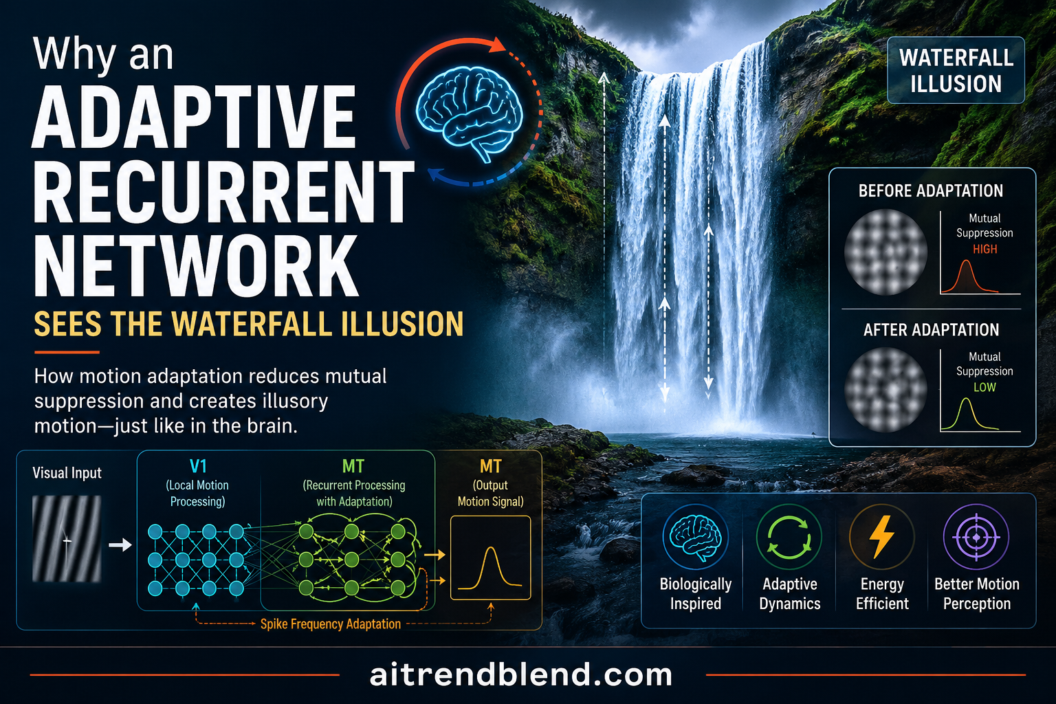
- The researchers trained two matched recurrent networks, MotionNet-R without adaptation and AdaptNet with it, on 60,000 natural image sequences from the Berkeley Segmentation Dataset.
- Only AdaptNet reproduced the waterfall illusion, overshooting into the opposite direction once a moving stimulus stopped.
- The overshoot traces back to a specific mechanism, a temporary collapse in mutual suppression between direction tuned units after one direction has been active for a while.
- AdaptNet used substantially less recurrent unit activity than MotionNet-R, at the cost of worse accuracy for constant motion and better accuracy right after a change.
- AdaptNet also reached its peak response two to three frames earlier than the non adaptive network, hinting that adaptation trades some steady state precision for faster reaction to change.
The problem with modeling adaptation instead of just modeling vision
Plenty of neural networks have been trained to estimate motion, and a fair number of them end up looking surprisingly biological once you probe their internal units. Simoncelli and Heeger built an influential model of area MT tuning back in 1998. Rust and colleagues followed with a more detailed V1 layer in 2006. Rideaux and Welchman showed in 2020 that a network trained purely on natural image statistics develops direction and speed tuning that lines up with what electrophysiologists find in monkey visual cortex. None of those models, though, tried to build in adaptation, the process by which a neuron’s response shrinks the longer it keeps firing to the same stimulus.
That is a real gap because adaptation is not a side detail of vision, it is closer to a design principle. It shows up at every timescale from milliseconds to hours, in every stage of the visual pathway, and it is the mechanism behind a long list of illusions and perceptual biases, the waterfall effect being the most famous. Researchers studying biological adaptation have had a hard time isolating its computational role because it is smeared across so many brain areas and cell types, with V1 and MT adapting at different rates and on different timescales. A model lets you strip that apart. You can build one network with adaptation and one without, hold everything else constant, and watch what changes.
That is exactly the comparison this paper runs. Two recurrent convolutional networks, identical in architecture, dropout, training data, and optimization, differing only in whether their V1 like and MT like units carry an adaptation variable that grows while a unit is active and slowly decays when it is not.
Why this matters beyond neuroscience
If adaptation genuinely buys a network lower energy use and faster reaction to change, that is a practical argument for adding similar mechanisms to production vision systems that run on limited power budgets, such as edge devices or always on cameras that mostly watch a static scene punctuated by brief events worth catching quickly.
Two networks, one difference
Shared architecture
Both MotionNet-R and AdaptNet share the same three stage structure. A two dimensional convolutional layer with sixteen 6 by 6 kernels plays the role of V1, taking two consecutive grayscale frames as separate input channels. A recurrent layer with a rectified linear activation plays the role of MT, integrating the convolutional output over time. A linear readout layer maps the recurrent activity onto an estimated horizontal and vertical velocity. Dropout at 0.3 sits after both the convolutional and recurrent layers for regularization, and it does not interact with the adaptation mechanism in either direction.
Training used 60,000 ten frame natural image sequences built with a sliding window over photographs from the Berkeley Segmentation Dataset, the same source used in the team’s earlier MotionNet work. Images were converted to grayscale, so each sequence carried only luminance information, and ten separate instances of each network were trained for thirty epochs apiece so the researchers could quantify variability across random initializations rather than reporting results from a single lucky run.
The adaptation mechanism itself
This is where AdaptNet diverges. Each unit in the V1 and MT layers carries an adaptation variable that behaves like a slow moving average of the unit’s own recent output. When a unit fires, its adaptation value grows. When it falls quiet, the adaptation value decays back down. That value gets subtracted from the unit’s pre activation before the result is passed forward and rectified.
Here \(s_t\) is the raw convolutional output at time \(t\), and \(a^{V1}_{t-1}\) is the accumulated V1 adaptation from the previous step. The adaptation rate \(\alpha^{V1}\) was set to 0.1 and the recovery rate \(\beta^{V1}\) to 0.1, meaning V1 units both build up and shed adaptation relatively gently. The MT layer follows the same pattern with its own pre activation \(p_t\), which combines the adapted V1 signal, the previous MT hidden state, and bias terms.
The MT adaptation rate \(\alpha^{MT}\) was set higher, at 0.2, while the recovery rate stayed at 0.1. That asymmetry between V1 and MT was a deliberate choice, matched to physiological findings that MT neurons in macaque adapt more strongly than V1 neurons under matched stimulus conditions, a pattern reported by Patterson and colleagues in 2014 and by Priebe and colleagues in earlier work on short term motion adaptation. MotionNet-R simply drops both equations and passes the raw rectified activity straight through.
Both networks learned to look like real visual cortex first
Before testing for the illusion, the authors checked whether either network actually behaved like a plausible model of V1 and MT in the first place. On that front both networks passed. Convolutional kernels came out looking like edge detectors or Gabor filters, with a phase shift between the two input channels that effectively builds a motion energy detector out of two static frames, the same trick used by classic V1 simple cell models. Speed tuning in the convolutional layer skewed toward slower speeds than the recurrent layer, matching the well documented difference between V1 and MT neurons in macaque, where MT cells respond to a broader and generally faster range of speeds.
The networks also reproduced a subtler and more diagnostic property, the shift from component motion selectivity in V1 to pattern motion selectivity in MT. When you show a V1 neuron a plaid made of two overlapping gratings moving in different directions, it tends to respond to the individual grating components. An MT neuron pools across V1 inputs and responds instead to the combined pattern direction, which is closer to what a person actually perceives when looking at a moving plaid. Both networks recreated this V1 to MT shift, and the authors note that this particular property emerges even in simpler networks without recurrence or adaptation, since it mainly depends on pooling signals across earlier units rather than on any timing mechanism.
Weight analysis added a third piece of evidence. Feedforward connections from V1 to MT units were stronger between units with similar direction tuning, consistent with motion pooling, and recurrent MT to MT connections showed the same pattern, positive between similarly tuned units and negative between oppositely tuned ones, a balance the authors compare to the excitatory and suppressive lateral connections documented in visual cortex.
The waterfall illusion, reproduced and explained
With the basic biological plausibility established, the authors ran the test that matters most for this paper. They built an eleven frame test sequence, two stationary frames to check for any baseline bias, three frames of motion to induce adaptation, then six stationary frames to look for an aftereffect.
MotionNet-R behaved the way you would expect from a network with no memory of sustained exposure. Its velocity estimate rose during the moving frames and settled smoothly back toward zero once the stimulus stopped. AdaptNet did something different. Once the motion ended, its estimate did not simply return to zero, it overshot into the opposite direction before recovering, exactly the signature of the waterfall illusion described in Mather and Harris’s account of the motion aftereffect.
The authors traced this directly to unit level activity in the recurrent MT layer. Before motion starts, units tuned to every direction respond about equally, holding a balanced baseline. Once motion begins, units tuned to that direction ramp up while units tuned to other directions get suppressed, consistent with the motion opponency mechanism described by Heeger and colleagues. When the motion stops, the units that had been most active are also the most adapted, so they recover more slowly, and for a brief window the previously suppressed population dominates the response. That temporary imbalance is read out by the linear layer as motion in the opposite direction, which is the illusion.
This mechanism lines up with a specific theoretical account that predates the paper by decades, going back to Barlow and Hill’s 1963 hypothesis that the waterfall phenomenon comes from a physiological imbalance rather than a purely perceptual or cognitive process, and echoed more recently by Grunewald and Lankheet and by Kohn and Movshon’s work on MT adaptation. What this paper adds is a working model where you can watch that imbalance happen unit by unit, rather than infer it indirectly from population recordings or psychophysics.
A side effect nobody was looking for
The authors also noticed that AdaptNet reacts to the onset of motion faster than MotionNet-R does. Measuring the number of frames each network needed to reach peak velocity estimation, AdaptNet consistently got there two to three frames sooner across a range of speeds. Their explanation is that adaptation reduces lateral suppression carried over from the previous stationary period, so direction tuned units have less resistance to overcome when a new stimulus arrives. MotionNet-R’s response instead builds gradually as it integrates information over consecutive frames, a pattern more suited to steady accumulation than rapid reaction.
Adaptation buys efficiency, but not for free
The paper’s second major comparison looks at energy use, using total recurrent unit activation as a proxy for metabolic cost, and prediction accuracy under two conditions, constant motion held steady across a sequence and motion that changes speed or direction periodically.
| Condition | MotionNet-R MSE | AdaptNet MSE | Statistical result |
|---|---|---|---|
| Constant motion | Lower error | Higher error | t(9) = negative 4.87, p = 4.29 times ten to the negative six |
| Motion with periodic change | Higher error | Lower error | t(9) = 10.09, p = 8.45 times ten to the negative twenty four |
| Recurrent activity, constant | Higher | Substantially lower | t(9) = 13.34, p = 9.07 times ten to the negative twenty four |
| Recurrent activity, with change | Higher | Substantially lower | t(9) = 159.3, p effectively zero |
Read that table as a trade rather than a straightforward win. AdaptNet is worse at holding a steady, accurate estimate of unchanging motion, which makes sense given that its units are quite literally fatiguing under sustained stimulation. But it is meaningfully better at estimating motion right after a change, and it does both things while using far less recurrent activity overall. The authors frame this as a real biological trade off, energy conserved by lower firing over time in exchange for reduced fidelity during long stretches of unchanging input, and point out that in nature this trade usually pays off because changing events tend to carry more ecological relevance than events that stay the same.
Key takeaway
Adding a simple, biologically inspired accumulate and decay rule to recurrent units did not just reproduce a known illusion. It produced a measurable, statistically consistent shift in what the network is good at, trading steady state accuracy for change detection and lower average activation, without changing the architecture in any other way.
Sensitivity to change, measured directly
To dig further into that trade, the authors ran a sensitivity test using nine frames at one speed followed by a tenth frame that either matched or changed. Fitting a sigmoid to each network’s accuracy across a range of final speeds, MotionNet-R showed a steeper curve for congruent sequences where the speed stayed the same throughout, which fits with its stronger performance on constant motion. AdaptNet showed the steeper curve for incongruent sequences where the final frame’s speed diverged from what came before, meaning it was more sensitive to the change itself. That result mirrors a broader idea in sensory neuroscience, that adaptation exists in part to amplify sensitivity to change at the expense of steady state precision, a point made across species by Fairhall and colleagues and more recently by Luczak and Kubo.
Key takeaway
The two networks are not simply better or worse versions of each other. MotionNet-R optimizes for tracking something that keeps moving the same way. AdaptNet optimizes for noticing when something changes. Which one you would actually want depends entirely on what your downstream task needs to catch.
What this means beyond one toy network
The authors are upfront that this is a small, deliberately constrained model, not a benchmark competitor, and they say as much rather than dressing it up as state of the art. The point was to isolate one mechanism, not to chase accuracy numbers against modern optical flow networks. Even so, the pattern they found lines up with a cluster of separate research threads that rarely get tested against each other in the same system. Efficiency gains from adaptation have been shown in spiking neural networks and adaptive exponential neuron models used in neuromorphic hardware. Change detection benefits from adaptation have been demonstrated behaviorally in mice performing visual change detection tasks. This paper is one of the few places those two benefits, lower energy use and higher change sensitivity, show up together inside a single trained artificial network built from natural image statistics rather than hand designed stimuli.
For anyone building vision systems with power constraints, the implication worth sitting with is not that adaptation makes a network strictly better. It is that adaptation reshapes what a network is good at in a specific and predictable direction, and that direction happens to match what a lot of real world monitoring tasks actually care about, catching the moment something changes rather than perfectly tracking something that already settled into a steady state.
Honest limitations
The adaptation mechanism used here is intentionally simple, a single accumulate and decay variable per unit, and the authors are direct about that being a simplification compared to the biological reality of adaptation, which involves neurotransmitter dynamics, ion channel kinetics, and modulatory input from other brain regions that this model does not attempt to capture. The training data, natural photographs from the Berkeley Segmentation Dataset turned into short synthetic motion sequences, gives the network a naturalistic visual diet but not the full variability of real world video. The authors also chose not to benchmark either network against modern optical flow or motion estimation systems, since the goal was isolating the effect of adding adaptation to a well understood baseline architecture rather than chasing state of the art numbers, and MotionNet-R’s own properties had already been validated in earlier work from the same lab. Readers should treat the reported magnitudes as informative about the direction of the effect rather than as numbers that will scale unchanged to larger, more complex production networks.
Complete PyTorch implementation
Below is a full, runnable implementation that follows the paper’s equations for both networks, along with a training loop skeleton and a smoke test on random dummy data so you can confirm the shapes and adaptation dynamics behave as described before running it on real sequences.
import torch
import torch.nn as nn
import torch.nn.functional as F

class AdaptiveConvLayer(nn.Module):
    """V1 like layer. Optionally applies accumulate and decay adaptation."""
    def __init__(self, in_channels=2, out_channels=16, kernel_size=6,
                 adapt=True, alpha=0.1, beta=0.1):
        super().__init__()
        self.conv = nn.Conv2d(in_channels, out_channels, kernel_size, stride=1)
        self.adapt = adapt
        self.alpha = alpha
        self.beta = beta

    def forward(self, x, a_prev):
        s = self.conv(x)
        if not self.adapt:
            return F.relu(s), None
        if a_prev is None:
            a_prev = torch.zeros_like(s)
        y = F.relu(s - a_prev)
        a_new = (1 - self.beta) * a_prev + self.alpha * y
        return y, a_new


class AdaptiveRecurrentCell(nn.Module):
    """MT like layer. Combines V1 input and previous hidden state."""
    def __init__(self, in_features, hidden_features,
                 adapt=True, alpha=0.2, beta=0.1):
        super().__init__()
        self.wx = nn.Linear(in_features, hidden_features)
        self.wh = nn.Linear(hidden_features, hidden_features)
        self.adapt = adapt
        self.alpha = alpha
        self.beta = beta

    def forward(self, y_v1, h_prev, a_prev):
        p = self.wx(y_v1) + self.wh(h_prev)
        if not self.adapt:
            r = F.relu(p)
            return r, r, None
        if a_prev is None:
            a_prev = torch.zeros_like(p)
        r = F.relu(p - a_prev)
        a_new = (1 - self.beta) * a_prev + self.alpha * r
        return r, r, a_new


class MotionEstimator(nn.Module):
    """Full network. Set adapt=False to recreate MotionNet-R, adapt=True for AdaptNet."""
    def __init__(self, adapt=True, img_size=32, kernel_size=6,
                 conv_channels=16, hidden_size=64, dropout=0.3):
        super().__init__()
        self.v1 = AdaptiveConvLayer(2, conv_channels, kernel_size,
                                     adapt=adapt, alpha=0.1, beta=0.1)
        conv_out = img_size - kernel_size + 1
        flat_features = conv_channels * conv_out * conv_out
        self.drop_v1 = nn.Dropout(dropout)
        self.mt = AdaptiveRecurrentCell(flat_features, hidden_size,
                                         adapt=adapt, alpha=0.2, beta=0.1)
        self.drop_mt = nn.Dropout(dropout)
        self.readout = nn.Linear(hidden_size, 2)
        self.hidden_size = hidden_size

    def forward(self, sequence):
        # sequence shape is batch, frames, height, width
        batch, frames, h, w = sequence.shape
        device = sequence.device
        h_state = torch.zeros(batch, self.hidden_size, device=device)
        a_v1 = None
        a_mt = None
        outputs = []
        for t in range(frames - 1):
            pair = torch.stack([sequence[:, t], sequence[:, t + 1]], dim=1)
            y_v1, a_v1 = self.v1(pair, a_v1)
            y_v1 = self.drop_v1(y_v1).flatten(1)
            r_mt, h_state, a_mt = self.mt(y_v1, h_state, a_mt)
            h_state = self.drop_mt(h_state)
            q = self.readout(h_state)
            outputs.append(q)
        return torch.stack(outputs, dim=1)


def motion_loss(pred, target):
    return F.mse_loss(pred, target)


def train_step(model, optimizer, sequence, target_velocity):
    model.train()
    optimizer.zero_grad()
    pred = model(sequence)
    # compare against ground truth velocity repeated across frames
    target = target_velocity.unsqueeze(1).expand(-1, pred.shape[1], -1)
    loss = motion_loss(pred, target)
    loss.backward()
    optimizer.step()
    return loss.item()


def evaluate(model, sequence, target_velocity):
    model.eval()
    with torch.no_grad():
        pred = model(sequence)
        target = target_velocity.unsqueeze(1).expand(-1, pred.shape[1], -1)
        loss = motion_loss(pred, target)
    return loss.item(), pred


if __name__ == "__main__":
    # smoke test on random dummy data, ten frame sequences, 32 by 32 grayscale
    torch.manual_seed(0)
    batch_size, frames, size = 4, 10, 32
    dummy_sequence = torch.randn(batch_size, frames, size, size)
    dummy_velocity = torch.randn(batch_size, 2)

    adaptnet = MotionEstimator(adapt=True)
    motionnet_r = MotionEstimator(adapt=False)

    opt_a = torch.optim.Adam(adaptnet.parameters(), lr=1e-3)
    opt_b = torch.optim.Adam(motionnet_r.parameters(), lr=1e-3)

    loss_a = train_step(adaptnet, opt_a, dummy_sequence, dummy_velocity)
    loss_b = train_step(motionnet_r, opt_b, dummy_sequence, dummy_velocity)

    print("AdaptNet dummy training loss", loss_a)
    print("MotionNet-R dummy training loss", loss_b)

    eval_loss, pred = evaluate(adaptnet, dummy_sequence, dummy_velocity)
    print("AdaptNet output shape", pred.shape)
    print("AdaptNet eval loss", eval_loss)
The smoke test builds one network with adaptation switched on and one with it switched off, runs a single training step on random noise for each, and prints the resulting shapes and losses so you can confirm the adaptation state is being carried correctly across frames before pointing the model at real motion sequences.
Conclusion
The core achievement here is narrow by design and stronger for it. Mohan and Rideaux did not set out to build a better motion estimator. They set out to isolate one mechanism, a simple accumulate and decay rule applied to V1 and MT like units, and check whether it was sufficient on its own to produce a well known perceptual illusion. It was, and the mechanism they found inside the trained network, a temporary collapse in mutual suppression between direction tuned populations, matches a decades old theoretical account of the waterfall effect that had mostly been argued from psychophysics and indirect neural recordings rather than watched directly inside a working system.
The conceptual shift worth sitting with is that adaptation is not just a source of illusions and quirks, it is a computational strategy with measurable trade offs that this paper actually quantifies. Lower energy use, worse tracking of unchanging input, better sensitivity to change, faster reaction time. Those four properties showed up together and consistently across ten independently trained instances of the network, which is a meaningfully stronger claim than a demonstration from a single lucky run.
Whether this transfers to domains outside vision is an open and genuinely interesting question. Adaptation like mechanisms already show efficiency gains in spiking neural networks built for neuromorphic hardware, and the change detection benefit documented here echoes findings in auditory and even vestibular adaptation research. A recurrent system built for any sensory stream that alternates between long stable periods and brief meaningful changes, audio event detection, sensor monitoring, even some financial time series, might see a similar trade between steady state precision and change sensitivity if a comparable accumulate and decay term were added to its recurrent units.
The honest limitations are worth repeating rather than glossing over. This is a small, two layer network trained on synthetic motion built from static photographs, tested against a simplified adaptation rule that does not capture the full biophysics of real neurons, and it was never meant to compete with modern optical flow systems on accuracy. The authors are explicit about all of that, and it is one of the more refreshing parts of the paper.
What stays with you after reading it is not a benchmark number. It is the image of a network that, given nothing but natural scenes and one extra term in its update equation, rediscovered on its own something a curious person notices the first time they watch a real waterfall and then look away.
Key takeaway
A single, biologically motivated adaptation rule was enough to make a recurrent network experience an illusion, trade accuracy for efficiency in a measurable way, and react faster to change, all from the same small architectural change.
Frequently asked questions
What is the waterfall illusion and why does it matter for this study
The waterfall illusion, also called the motion aftereffect, happens when prolonged exposure to motion in one direction makes a subsequently viewed stationary scene appear to move in the opposite direction. It matters here because it is one of the clearest behavioral signatures of motion adaptation in biological vision, and reproducing it inside a trained artificial network is strong evidence that the network’s adaptation mechanism is doing something functionally similar to what happens in real visual cortex.
What is the actual difference between MotionNet-R and AdaptNet
The two networks share identical architecture, training data, and optimization settings. The only difference is that AdaptNet’s V1 and MT like units carry an adaptation variable that accumulates while a unit is active and decays when it is not, and that variable is subtracted from the unit’s input before rectification. MotionNet-R skips this step entirely.
Does adaptation make the network more accurate overall
No, and the paper is direct about that. AdaptNet was less accurate than MotionNet-R for constant, unchanging motion, but more accurate right after a change in motion direction or speed. The trade off is the point of the paper rather than a flaw in it.
Why does AdaptNet use less energy than MotionNet-R
The researchers measured total recurrent unit activation as a proxy for the metabolic cost of sustaining a neural representation. Because adaptation suppresses a unit’s response the longer it stays active, AdaptNet’s recurrent layer produced significantly lower total activity than MotionNet-R across both constant and changing motion conditions.
Is this network meant to compete with modern optical flow models
No. The authors describe both networks as intentionally small and constrained, built to isolate the effect of adding adaptation to a well understood baseline architecture rather than to chase state of the art accuracy against contemporary motion estimation systems.
Could this adaptation mechanism be applied outside motion processing
The paper only tests motion estimation, but the underlying mechanism, an accumulate and decay term subtracted from a recurrent unit’s input, is architecture agnostic. It could plausibly be tested in any recurrent system that processes a mostly steady signal punctuated by occasional meaningful changes, though that extension was not tested in this study.
Read the full study for the complete statistical results, additional supplementary figures, and the code repository.
Read the paper View the codeThroughout this piece we also link back to our broader coverage of computer vision research on aitrendblend.com.
Mohan, V., and Rideaux, R. Energy efficiency and sensitivity benefits in a motion processing adaptive recurrent neural network. Neural Networks, 191, 107834, 2025. https://doi.org/10.1016/j.neunet.2025.107834
This analysis is based on the published paper and an independent evaluation of its claims.