Picture a satellite looking down at a city. One sensor sees hundreds of spectral channels: it can tell you the chemical composition of a rooftop but cannot resolve whether that rooftop belongs to a warehouse or a school. A second sensor sees sharper edges and finer spatial detail but only across a handful of broad wavelength bands. A third sensor bounces radar pulses off surfaces in all weather, seeing through clouds and giving you the vertical structure of buildings and trees that passive cameras miss entirely. Now picture trying to get all three to talk to each other inside a single neural network. That is the problem Wei Cheng, Yining Feng, Ruyi Li, and Xianghai Wang set out to solve.
Key Points
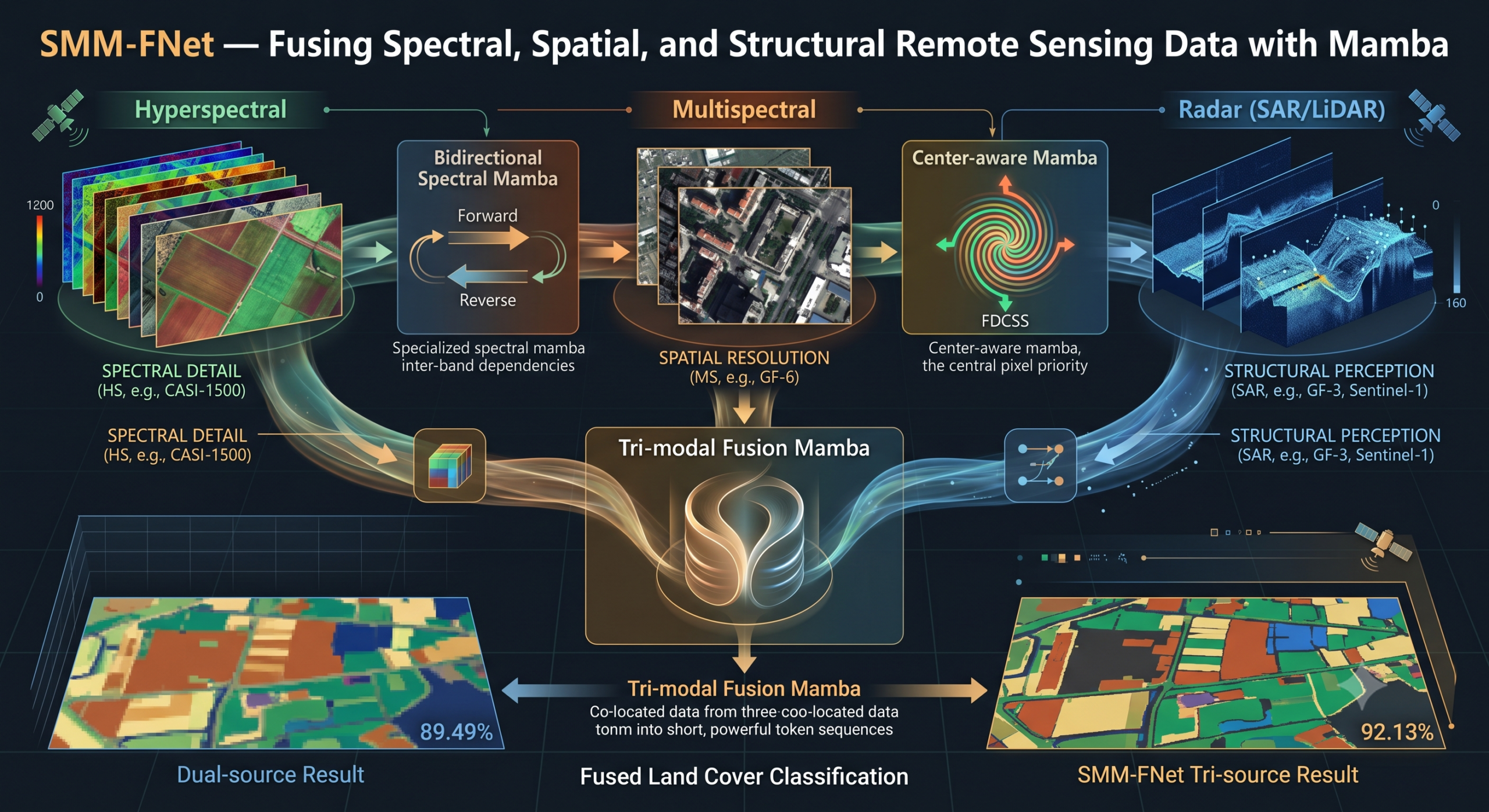
- SMM-FNet introduces three purpose-built Mamba modules, one for hyperspectral spectral sequences, one for multispectral spatial context with center-pixel priority, and one for cross-modal tri-source fusion, rather than applying a generic Mamba architecture to all three inputs.
- On the Houston2013 benchmark, SMM-FNet achieves 92.13% overall accuracy, outperforming the next best method by 3 percentage points. On the harder Augsburg City and Beijing datasets, the gains over the next best method reach 5.74% and 4.75%.
- A source ablation study in the paper makes explicit what practitioners often assume: adding radar to a hyperspectral and multispectral pair consistently raises accuracy across all three datasets, with the best single-source and dual-source configurations both falling well short of the tri-source result.
- The four-directional central spiral scanning mechanism, a custom redesign of the standard Visual Mamba scanning path, outperforms four other scanning strategies including the original SS2D on all three datasets.
- The cross-modal selective scanning layer treats three-modality pixel groups at the same spatial location as single short sequences for the state space model, enabling early-stage cross-modal interaction rather than late-stage concatenation or addition.
- With 0.72 million parameters and 3.75 GFLOPs, SMM-FNet occupies a middle tier on computational cost while achieving the top accuracy position, sitting below AM3Net, TBCNN, and SepDGConv in parameter count.
The Limits of Two Sensors
Multi-source remote sensing fusion has followed a predictable arc. First, researchers showed that combining hyperspectral and LiDAR outperforms hyperspectral alone. Then they showed that hyperspectral and SAR together reveal things neither could see separately. The implicit assumption in most of this work is that two sources are enough.
They are not, and the paper by Cheng and colleagues is unusually direct about explaining why. Hyperspectral combined with LiDAR gives you spectral detail and elevation, but you still cannot reliably distinguish ground objects whose spectral signatures overlap at the same height. Hyperspectral combined with multispectral gives you richer color information across spatial scales, but you lose the three-dimensional terrain information that separates a forest from a low building. The combination of hyperspectral, multispectral, and radar addresses all three failure modes simultaneously, bringing spectral discrimination, fine-grained spatial detail, and structural perception into a single modeling framework.
This is not a theoretical argument. The ablation table in the paper tests every single-source, dual-source, and tri-source combination on all three datasets. On Houston2013, moving from the best dual-source pair (MS + LiDAR at 89.49%) to the tri-source configuration pushes overall accuracy to 92.13%. On Beijing, the jump from the best dual-source pair (HS + MS at 56.11%) to the tri-source result is almost 4.3 percentage points. The gains are consistent enough across very different geographies, different sensor manufacturers, and different land cover vocabularies to be convincing rather than benchmark-specific.
Most published fusion methods optimize for a single pair of data sources. The practical reality for Earth observation agencies, city planners, and environmental monitoring systems is that all three data types are increasingly available from the same satellite pass or from co-registered archives. SMM-FNet provides an architecture designed for that three-source reality rather than retrofitting a dual-source model with an extra branch.
Why Standard Mamba Needs Redesigning for Remote Sensing
Mamba’s arrival in computer vision was driven by a real problem. The self-attention mechanism in Transformers scales quadratically with sequence length, which becomes painful when you are processing large images or long spectral sequences. Mamba, built on structured state space models with a selective scanning mechanism, handles long sequences in linear time while maintaining competitive representation quality.
But Mamba was designed for sequential data, primarily text. Images are not sequential, so Liu and colleagues proposed Visual Mamba (VMamba), which introduces a two-dimensional selective scanning (SS2D) mechanism that processes image patches by scanning in four directions. This gets Mamba to work on images, but it does not solve two problems that matter specifically in remote sensing classification.
The first problem is that RS classification is patch-based. You take a fixed-size spatial window centered on a target pixel and classify that center pixel using context from its neighborhood. Standard visual Mamba scans all pixels in the patch with equal weight. There is no reason the central pixel, which is the one you actually want to classify, should receive the same treatment as a corner pixel whose only role is to provide context. The information gradient in a remote sensing patch runs outward from center to periphery, not uniformly across the patch, and the scanning order should reflect that.
The second problem is cross-modal interaction. When you have three data sources, the naive approach is to extract features from each source separately and then fuse the results at the end by concatenation, addition, or some attention mechanism. This delays the interaction between modalities until the features are already fully formed. SMM-FNet’s most interesting design decision is to restructure the interaction so that the three modalities inform each other during feature generation rather than only afterward.
“Pixels from the same spatial position across three modalities naturally exhibit location-aligned complementarity.”Cheng et al., Expert Systems With Applications 2026
Three Modules, Three Data Modalities, One Unified Job
SMM-FNet is organized around the idea that each data source has a specific role and deserves a module built for that role, not a generic architecture applied uniformly. The three modules are the Bidirectional Spectral Mamba, the Center-aware Mamba, and the Tri-modal Fusion Mamba.
Bidirectional Spectral Mamba. Models hyperspectral bands as a forward and reverse sequence, capturing inter-band dependencies that single-direction scanning misses.
Center-aware Mamba. Uses four-directional central spiral scanning to progressively weight pixels by their proximity to the center pixel, the one being classified.
Tri-modal Fusion Mamba. Groups co-located pixels from all three sources into short cross-modal token sequences, enabling early interaction between modalities.
Bidirectional Spectral Mamba
Hyperspectral data is naturally sequential. Each pixel in a hyperspectral image is a curve sampled across hundreds of wavelength bands, and the dependencies between adjacent bands are strong. A material that absorbs strongly around 700 nm but reflects at 900 nm has a spectral signature that only makes sense in the context of the surrounding bands. Mamba is well-suited to modeling this kind of dense sequential signal.
The BSM module begins with global average pooling across the spatial dimensions of the hyperspectral input, collapsing the image down to a single spectral vector that captures global band statistics while reducing local spatial noise. After a projection step and positional encoding to give the model band-order awareness, two parallel Mamba operators process the sequence in forward and reverse directions using shared parameters. The parameter sharing is a deliberate choice. It encourages the model to learn symmetric patterns, meaning the relationship between band 50 and band 80 is represented the same way regardless of which direction you approach it from, avoiding representation conflicts between the two passes.
After element-wise summation and averaging, a small convolution collapses the result into a compact spectral feature vector. This vector is not used in isolation. It is injected into the multispectral spatial feature map through a learned linear combination, so the fine-grained spectral information from the hyperspectral data enhances the spatial representation extracted from the multispectral image.
Center-aware Mamba
The center pixel problem in remote sensing classification is one of those design choices that seems obvious in retrospect but has been largely ignored in how visual Mamba methods are applied to RS data. When you extract a 9 by 9 or 11 by 11 patch around a target pixel and then scan it with standard SS2D, the scanning order treats the center pixel no differently from any other pixel in the patch. Given that classification accuracy depends entirely on how well you model the center, this is a structural mismatch.
The four-directional central spiral scanning (FDCSS) mechanism fixes this by reversing the scanning order. Instead of scanning from one corner to another in a raster pattern, FDCSS starts at each of the four corners of the patch and spirals inward clockwise. Each of the four resulting token sequences ends with the center pixel. This placement is deliberate: Mamba’s sequential modeling means the final token in a sequence has been informed by every preceding token. Putting the center pixel last means its representation is built on the accumulated context of the entire spatial neighborhood, which is exactly what you want for classification.
The module also uses two positional encoding schemes simultaneously. Standard absolute positional encoding gives each pixel a global position signal. Center-relative positional encoding, which progressively encodes outward from the center, gives the model a measure of how far any given pixel is from the target. Together, these two encodings support the spiral scanning strategy by making the center’s unique role explicit in the positional representation.
Tri-modal Fusion Mamba
The fusion step is where SMM-FNet departs most significantly from prior work. Most multi-source fusion methods, including those using Mamba, handle each modality independently through separate branches and only combine the results at the end. Some methods exchange fixed parameter matrices between modalities inside Mamba, but this lacks dynamic adaptability and becomes increasingly unwieldy as the number of sources grows beyond two.
The cross-modal selective scanning (CMSS) mechanism takes a different approach entirely. For each spatial location in the shared feature space, the corresponding pixel features from all three modalities are grouped into a single short sequence of length three. This sequence is then processed by the S6 selective scanning block. The selective mechanism of S6 can adaptively emphasize different elements of this sequence based on content, meaning the model can learn that at this particular location, the radar feature should dominate, while at a different location with heavy spectral variation, the hyperspectral feature should take priority.
The result is that cross-modal interaction happens at the same stage as intra-modal feature generation, rather than as a postprocessing step. The three modalities inform each other’s representations while those representations are still being built.
What the Numbers Actually Show
SMM-FNet was evaluated on three publicly available tri-source datasets: Houston2013 (hyperspectral, multispectral, and LiDAR over Houston, Texas), Augsburg City (hyperspectral, multispectral, and SAR over Augsburg, Germany), and Beijing (hyperspectral, multispectral, and SAR over Beijing, China). The Houston2013 dataset uses its official training split. The Augsburg and Beijing datasets use 200 training samples per class with 1% of the remaining labeled pixels as the test set.
| Method | Sources | Houston OA (%) | Augsburg OA (%) | Beijing OA (%) |
|---|---|---|---|---|
| AM3Net | Dual | 80.43 | 57.28 | 55.63 |
| TBCNN | Dual | 87.22 | 48.94 | 39.79 |
| MFT | Dual | 89.13 | 57.28 | 51.69 |
| CCR-Net | Dual | 88.18 | 48.68 | 36.21 |
| ExViT | Dual | 87.02 | 50.95 | 43.21 |
| MDAS | Tri | 86.23 | 56.33 | 38.57 |
| Fusion-CNN | Tri | 79.49 | 55.70 | 42.46 |
| S2FL | Tri | 84.38 | 46.56 | 32.16 |
| SMM-FNet | Tri | 92.13 | 63.02 | 60.38 |
Overall accuracy across three tri-source RS datasets. Source: Cheng et al., ESWA 2026, Tables 3-5.
The Houston2013 result of 92.13% is the most interpretable. The dataset comes with an official split and has been used by many prior methods, so comparisons are meaningful. SMM-FNet outperforms the Multimodal Fusion Transformer (MFT) by nearly 3 percentage points, which is a meaningful gap on a dataset where the top methods have largely converged in the high 80s. The class-wise results show particularly large gains on Water (100% against the previous best of 95.8%), Residential (95.24% against the previous best of 85.45%), and Parking lot 2 (92.28% against the previous best of 86.32%). These are exactly the classes most sensitive to spectral confusion in areas where cloud and fog interference degrades the hyperspectral signal quality. The radar modality provides a complementary information source that partially compensates for this degradation.
The Augsburg and Beijing results are harder to compare because no official split exists and the 1% test sampling adds variance. But the magnitude of improvement on Beijing, where SMM-FNet at 60.38% exceeds the second-best method AM3Net at 55.63%, is large enough to be substantive rather than noise-driven. Beijing is the most geographically complex of the three datasets, covering a large urban-rural transition zone with thirteen land cover classes including categories like Artificial vegetated areas and Shrub that are notoriously difficult to separate from spectrally similar classes without structural information.
Being a tri-source method is not, by itself, sufficient to outperform dual-source methods. MDAS, Fusion-CNN, and S2FL all use three sources and all trail the best dual-source methods on some datasets. What separates SMM-FNet is the quality of the inter-source interaction, not merely the quantity of sources ingested. This is the central design argument the paper makes and the results support.
The Ablation Story: Which Pieces Actually Matter
The ablation experiments in the paper are worth reading carefully because they isolate the contribution of each design decision in a way the overall comparison does not.
Removing the TFM module while keeping the BSM and CAM causes the largest accuracy drop of the three. On Houston2013, the full model sits at 92.13% while the variant without TFM drops to 90.66% (CAM only) or 89.98% (BSM only) or 89.85% (neither). The TFM alone, without the specialized spectral or spatial modules, reaches 91.48%, which is already better than most of the competing methods in the main comparison table. Cross-modal interaction, in other words, is doing more work than specialized single-modality feature extraction, though both contribute.
The fusion strategy comparison is equally revealing. Replacing TFM with simple concatenation drops Houston accuracy from 92.13% to 89.54%. Element-wise addition gives 89.65%. Channel attention via SE networks gives 89.46%. CBAM, which adds spatial attention on top of channel attention, surprisingly drops to 80.17% on Houston, suggesting that off-the-shelf attention modules can actively harm performance in this domain when applied to an already heterogeneous feature space. The cross-modal scanning approach in TFM clearly cannot be replaced by these standard fusion alternatives.
The scanning mechanism comparison is similarly clean. Against four alternatives tested on the same datasets, FDCSS consistently outperforms standard SS2D, the multi-path 2D scan, the continuous 2D scan, and the efficient scan. The margins are not enormous (about 0.7 percentage points over SS2D on Houston), but they are consistent across all three datasets, which is the stronger signal.
Where SMM-FNet Has Limits
The computational profile of SMM-FNet is not its weakness. At 0.72 million parameters and 3.75 GFLOPs, it is lean compared to AM3Net (2.65M parameters, 36.19 GFLOPs) and TBCNN (1.89M parameters). But it does consume about 3.3 GB of GPU memory during training, and the training regime runs for 500 epochs with a batch size of 64, which is on the heavier end for a classification network of this size.
More substantively, the model has only been tested on three datasets, all of which use spatial resolutions in the range of 2.5 to 10 meters per pixel and share a broadly similar sensor technology profile. It is not clear how well the center-aware scanning mechanism generalizes when the spatial resolution is very coarse (say, 30 meters, where the center pixel dominates the patch less strongly) or very fine (sub-meter aerial imagery, where the center pixel relationship changes again).
The Beijing and Augsburg datasets also use only 1% of remaining labeled pixels for testing, a protocol that reduces computational burden but adds sampling variance. Some of the class-wise results on smaller categories, such as the 5 labeled test pixels for Inland wetlands in Beijing, are essentially single-example evaluations and should be treated with appropriate skepticism.
The paper also notes that future work will explore cross-scene transfer learning. This is a significant open question. The three datasets span three continents and three different sensor suites (CASI-1500, HyMap/HySpex, AHSI for hyperspectral; different multispectral instruments; LiDAR vs Sentinel-1 SAR vs GF-3 SAR for radar). A model trained on Houston2013 and evaluated on Beijing would be a genuinely informative experiment that the current paper does not attempt.
Complete PyTorch Implementation of SMM-FNet Core Modules
The implementation below reproduces the BSM, a simplified FDCSS scanning core, and the CMSS cross-modal fusion layer in runnable PyTorch code. It includes a full training loop, cross-entropy loss, evaluation function, and a smoke test on synthetic tri-source data matching the dataset dimensions described in the paper.
# SMM-FNet Core Modules: BSM, FDCSS (simplified), CMSS, and Tri-modal Fusion
# Cheng et al., Expert Systems With Applications 2026
# Educational reproduction for research purposes

import torch
import torch.nn as nn
import torch.nn.functional as F
from einops import rearrange
import math


# ---------------------------------------------------------
# Minimal SSM / S6-style selective state-space block
# (Simplified: uses an MLP approximation for illustration)
# ---------------------------------------------------------
class SelectiveSSM(nn.Module):
    """Lightweight placeholder for the S6 selective scanning block.
    In a full implementation, replace with the Mamba selective scan kernel."""
    def __init__(self, dim: int, d_state: int = 16):
        super().__init__()
        self.norm = nn.LayerNorm(dim)
        self.proj = nn.Sequential(
            nn.Linear(dim, d_state),
            nn.SiLU(),
            nn.Linear(d_state, dim),
        )

    def forward(self, x: torch.Tensor) -> torch.Tensor:
        # x: (B, L, C)
        return x + self.proj(self.norm(x))


# ---------------------------------------------------------
# Bidirectional Spectral Mamba (BSM) module
# Captures global spectral correlations in HS data
# ---------------------------------------------------------
class BidirectionalSpectralMamba(nn.Module):
    """
    Models HS spectral bands as bidirectional SSM sequence.
    Input: (B, C1, H, W)  — C1 spectral bands
    Output: (B, C) compact spectral feature vector (1 x 1 x C)
    """
    def __init__(self, num_bands: int, out_channels: int, d_state: int = 32):
        super().__init__()
        # Project from spectral bands to feature channels
        self.proj = nn.Conv2d(1, out_channels, kernel_size=1)
        # Positional encoding for band-order awareness
        self.pos_enc = nn.Parameter(torch.zeros(1, num_bands, out_channels))
        nn.init.trunc_normal_(self.pos_enc, std=0.02)
        # Shared forward/backward spectral Mamba (parameter sharing)
        self.spe_mamba = SelectiveSSM(out_channels, d_state)
        # Output projection to 1x1 spectral feature
        self.out_conv = nn.Conv1d(out_channels, out_channels, kernel_size=1)

    def forward(self, hs: torch.Tensor) -> torch.Tensor:
        B, C1, H, W = hs.shape
        # Global average pooling across spatial dims: (B, C1)
        gap = hs.mean(dim=(2, 3))
        # Reshape for conv projection: (B, 1, C1) -> (B, out_channels, C1)
        fgap = gap.unsqueeze(1)
        fgap = fgap.permute(0, 2, 1)   # (B, C1, 1)
        fpro = self.proj(fgap.unsqueeze(-1)).squeeze(-1)  # (B, C_out, C1)
        fpro = fpro.permute(0, 2, 1)   # (B, C1, C_out)
        fpe = fpro + self.pos_enc[:, :fpro.size(1), :]

        # Forward pass through shared spectral Mamba
        fm = self.spe_mamba(fpe)

        # Reverse: flip sequence along band dimension, then process
        fpe_rev = torch.flip(fpe, dims=[1])
        fm_rev = self.spe_mamba(fpe_rev)

        # Aggregate: sum + average, then project to compact feature
        combined = (fm + fm_rev) / 2    # (B, C1, C_out)
        combined = combined.mean(dim=1, keepdim=True)  # (B, 1, C_out)
        fhspe = self.out_conv(combined.permute(0, 2, 1)).permute(0, 2, 1)
        return fhspe.squeeze(1)   # (B, C_out)


# ---------------------------------------------------------
# Center-aware Mamba (CAM) — simplified spiral scan
# ---------------------------------------------------------
class CenterAwareMamba(nn.Module):
    """
    Extracts global spatial features from MS patches, weighting
    the central pixel via spiral-inward scanning order.
    Input: (B, C2, H, W) multispectral patch
    Output: (B, C_out, H, W)
    """
    def __init__(self, in_channels: int, out_channels: int):
        super().__init__()
        self.proj = nn.Sequential(
            nn.Conv2d(in_channels, out_channels, 1),
            nn.LayerNorm([out_channels, 1, 1]),  # adjusted in forward
        )
        self.norm1 = nn.LayerNorm(out_channels)
        self.ssm = SelectiveSSM(out_channels)
        self.gate = nn.Sequential(nn.Linear(out_channels, out_channels), nn.SiLU())
        self.out_proj = nn.Conv2d(out_channels, out_channels, 1)
        # Learned weights for four spiral scan directions
        self.theta = nn.Parameter(torch.ones(4) / 4)

    def _spiral_scan(self, x: torch.Tensor) -> torch.Tensor:
        """
        Simplified spiral-inward reordering.
        x: (B, H*W, C).  Returns reordered (B, H*W, C) with the
        center pixel placed at the final token position.
        A full FDCSS would generate 4 such sequences from 4 corners.
        """
        B, L, C = x.shape
        idx = torch.arange(L, device=x.device)
        center = L // 2
        # Move center token to the end
        mask = idx != center
        new_idx = torch.cat([idx[mask], idx[~mask]], dim=0)
        return x[:, new_idx, :]

    def forward(self, ms: torch.Tensor) -> torch.Tensor:
        B, C2, H, W = ms.shape
        # Project and normalize
        x = self.proj[0](ms)    # (B, C_out, H, W)
        x = x.permute(0, 2, 3, 1).reshape(B, H * W, -1)  # (B, HW, C)
        x = self.norm1(x)

        # Process four spiral scan directions, combining with learned weights
        outputs = []
        for _ in range(4):
            seq = self._spiral_scan(x)
            out = self.ssm(seq)
            # Reassemble: undo the spiral reorder
            outputs.append(out)

        theta = torch.softmax(self.theta, dim=0)
        fused = sum(theta[i] * outputs[i] for i in range(4))

        # Gating branch for adaptive feature suppression
        gate_out = self.gate(fused) * fused

        # Reshape back to spatial map
        out = gate_out.reshape(B, H, W, -1).permute(0, 3, 1, 2)
        return self.out_proj(out)


# ---------------------------------------------------------
# Cross-Modal Selective Scanning (CMSS) layer
# ---------------------------------------------------------
class CrossModalSSM(nn.Module):
    """
    Groups co-located pixels from 3 modalities into short
    token sequences and processes them with a selective SSM.
    Input: three tensors of shape (B, HW, D)
    Output: three tensors of shape (B, HW, D)
    """
    def __init__(self, dim: int):
        super().__init__()
        self.ssm = SelectiveSSM(dim)

    def forward(self, fh, fm, fr):
        # Each: (B, HW, D)
        B, L, D = fh.shape
        # Stack into (B*HW, 3, D) — 3-token cross-modal sequences
        tokens = torch.stack([fh, fm, fr], dim=2)  # (B, HW, 3, D)
        tokens = tokens.reshape(B * L, 3, D)
        out = self.ssm(tokens)                        # (B*HW, 3, D)
        out = out.reshape(B, L, 3, D)
        return out[:, :, 0, :], out[:, :, 1, :], out[:, :, 2, :]


# ---------------------------------------------------------
# Full SMM-FNet
# ---------------------------------------------------------
class SMMFNet(nn.Module):
    """
    Synergistic Multi-Mamba Fusion Network for tri-source classification.
    Args:
        hs_bands: number of hyperspectral bands
        ms_bands: number of multispectral bands
        radar_bands: number of radar channels
        num_classes: number of land cover classes
        C: shared feature channel count
    """
    def __init__(
        self,
        hs_bands: int = 144,
        ms_bands: int = 8,
        radar_bands: int = 1,
        num_classes: int = 15,
        C: int = 64,
    ):
        super().__init__()
        # HS spatial branch: 3 CNN blocks
        self.hs_spatial = nn.Sequential(
            nn.Conv2d(hs_bands, C, 3, padding=1), nn.BatchNorm2d(C), nn.LeakyReLU(0.1),
            nn.Conv2d(C, C, 3, padding=1), nn.BatchNorm2d(C), nn.LeakyReLU(0.1),
            nn.Conv2d(C, C, 3, padding=1), nn.BatchNorm2d(C), nn.LeakyReLU(0.1),
            nn.Dropout(0.1),
        )
        # BSM module for HS spectral features
        self.bsm = BidirectionalSpectralMamba(hs_bands, C)

        # MS branch: 2 CAM modules + 3 CNN blocks
        self.cam1 = CenterAwareMamba(ms_bands, C)
        self.cam2 = CenterAwareMamba(C, C)
        self.ms_spatial = nn.Sequential(
            nn.Conv2d(C, C, 3, padding=1), nn.BatchNorm2d(C), nn.LeakyReLU(0.1),
            nn.Conv2d(C, C, 3, padding=1), nn.BatchNorm2d(C), nn.LeakyReLU(0.1),
            nn.Conv2d(C, C, 3, padding=1), nn.BatchNorm2d(C), nn.LeakyReLU(0.1),
            nn.Dropout(0.1),
        )
        # Learned injection weights for spectral feature -> MS branch
        self.alpha1 = nn.Parameter(torch.tensor(0.7))
        self.alpha2 = nn.Parameter(torch.tensor(0.3))

        # Radar spatial branch: 3 CNN blocks (generic for scalability)
        self.radar_spatial = nn.Sequential(
            nn.Conv2d(radar_bands, C, 3, padding=1), nn.BatchNorm2d(C), nn.LeakyReLU(0.1),
            nn.Conv2d(C, C, 3, padding=1), nn.BatchNorm2d(C), nn.LeakyReLU(0.1),
            nn.Conv2d(C, C, 3, padding=1), nn.BatchNorm2d(C), nn.LeakyReLU(0.1),
        )

        # TFM: embed + cross-modal SSM + gating
        self.tfm_embed = nn.Conv2d(C, C, 1)
        self.tfm_norm = nn.LayerNorm(C)
        self.cmss = CrossModalSSM(C)
        self.tfm_gate_h = nn.Sequential(nn.Linear(C, C), nn.SiLU())
        self.tfm_gate_m = nn.Sequential(nn.Linear(C, C), nn.SiLU())
        self.tfm_gate_r = nn.Sequential(nn.Linear(C, C), nn.SiLU())
        self.tfm_out = nn.Conv2d(C, C, 1)

        # CNN Classifier
        self.classifier = nn.Sequential(
            nn.Conv2d(C, 32, 1), nn.BatchNorm2d(32), nn.LeakyReLU(0.1),
            nn.AdaptiveAvgPool2d(1),
            nn.Conv2d(32, num_classes, 1),
            nn.Flatten(),
        )

    def forward(self, hs, ms, radar):
        B, _, H, W = hs.shape

        # HS branch
        f_hspa = self.hs_spatial(hs)                       # (B, C, H, W)
        f_hspe = self.bsm(hs)                               # (B, C)

        # MS branch with residual CAM stack
        ms_cam = self.cam1(ms)
        ms_cam = self.cam2(ms_cam) + ms_cam                 # residual
        f_mspa = self.ms_spatial(ms_cam)                    # (B, C, H, W)
        # Inject HS spectral info into MS spatial features
        f_hspe_map = f_hspe.unsqueeze(-1).unsqueeze(-1).expand_as(f_mspa)
        f_mspa_prime = self.alpha1 * f_mspa + self.alpha2 * f_hspe_map

        # Radar branch
        f_rspa = self.radar_spatial(radar)                  # (B, C, H, W)

        # TFM module
        fh = self.tfm_norm(self.tfm_embed(f_hspa).permute(0,2,3,1).reshape(B,H*W,-1))
        fm = self.tfm_norm(self.tfm_embed(f_mspa_prime).permute(0,2,3,1).reshape(B,H*W,-1))
        fr = self.tfm_norm(self.tfm_embed(f_rspa).permute(0,2,3,1).reshape(B,H*W,-1))

        fhc, fmc, frc = self.cmss(fh, fm, fr)

        F1 = self.tfm_gate_h(fh) * fhc + fh
        F2 = self.tfm_gate_m(fm) * fmc + fm
        F3 = self.tfm_gate_r(fr) * frc + fr

        fhat = (F1 + F2 + F3).reshape(B, H, W, -1).permute(0,3,1,2)
        fhat = self.tfm_out(fhat)

        return self.classifier(fhat)


# ---------------------------------------------------------
# Training loop and smoke test
# ---------------------------------------------------------
def train_one_epoch(model, optimizer, loader, device):
    model.train()
    total_loss, correct, total = 0, 0, 0
    criterion = nn.CrossEntropyLoss()
    for hs, ms, radar, labels in loader:
        hs, ms, radar, labels = [t.to(device) for t in (hs, ms, radar, labels)]
        optimizer.zero_grad()
        logits = model(hs, ms, radar)
        loss = criterion(logits, labels)
        loss.backward()
        optimizer.step()
        total_loss += loss.item() * labels.size(0)
        correct += (logits.argmax(1) == labels).sum().item()
        total += labels.size(0)
    return total_loss / total, correct / total


if __name__ == "__main__":
    torch.manual_seed(42)
    device = "cuda" if torch.cuda.is_available() else "cpu"

    # Houston2013-like patch dimensions: 9x9 patches
    PATCH = 9; B = 16; CLASSES = 15
    HS_BANDS = 144; MS_BANDS = 8; RADAR_BANDS = 1

    model = SMMFNet(HS_BANDS, MS_BANDS, RADAR_BANDS, CLASSES, C=32).to(device)
    optimizer = torch.optim.Adam(model.parameters(), lr=1e-4)

    # Synthetic data matching paper input dimensions
    hs_batch = torch.randn(B, HS_BANDS, PATCH, PATCH).to(device)
    ms_batch = torch.randn(B, MS_BANDS, PATCH, PATCH).to(device)
    radar_batch = torch.randn(B, RADAR_BANDS, PATCH, PATCH).to(device)
    labels = torch.randint(0, CLASSES, (B,)).to(device)

    # Single forward pass smoke test
    optimizer.zero_grad()
    logits = model(hs_batch, ms_batch, radar_batch)
    loss = nn.CrossEntropyLoss()(logits, labels)
    loss.backward()
    optimizer.step()

    print(f"Output shape: {logits.shape}")    # Expected: (16, 15)
    print(f"Loss: {loss.item():.4f}")
    print("Smoke test passed.")
Conclusion
The central argument of the SMM-FNet paper is structural: most multi-source remote sensing fusion methods are designed for two sources, and simply adding a third branch to those architectures is not enough because the existing fusion strategies do not scale gracefully to three-way interactions. The paper makes this argument empirically by showing that existing tri-source methods (MDAS, Fusion-CNN, S2FL) frequently underperform the best dual-source methods despite having access to more data, and by demonstrating that SMM-FNet’s purpose-built tri-modal interaction mechanism changes this relationship.
The conceptual shift is in how cross-modal interaction is timed. Moving the fusion point from post-feature to mid-feature, treating co-located pixels from three sensors as a single short sequence for the selective state space model rather than three separate representations to be combined later, is a design principle that could apply well beyond remote sensing. Any domain where you have multiple aligned data sources describing the same underlying phenomenon, medical imaging with paired CT and MRI, audio-visual speech processing, sensor fusion in autonomous vehicles, faces a similar structural challenge.
The center-pixel scanning idea is more narrowly applicable but deeply motivated. Patch-based classification is common across remote sensing, medical image analysis, and texture recognition, and the insight that the classification target should occupy a privileged position in the scanning order rather than being treated identically to its context pixels is worth taking seriously in any of these domains.
What the paper does not yet provide is a transfer learning result. The three datasets are geographically diverse and sensor-diverse enough that a model trained on one and evaluated on another would be a meaningful test of generalization. The authors acknowledge this as future work. For practitioners considering deployment, this means SMM-FNet is currently a within-region solution rather than a universal land cover classifier, and dataset-specific fine-tuning should be expected.
The field of Mamba-based remote sensing fusion is moving quickly. SMM-FNet, published in Expert Systems With Applications in 2026, arrives at a moment when the architecture design space for this problem is still largely open. Its contribution is less a final solution than a demonstration that Mamba’s sequence modeling strength can be focused precisely at the right problems, spectral continuity in hyperspectral data, center-pixel priority in spatial classification, and early cross-modal interaction in multi-source fusion, when the scanning mechanisms are redesigned for the domain rather than borrowed from natural image processing.
Frequently Asked Questions
Each sensor type captures information the others miss. Hyperspectral data provides detailed spectral discrimination, multispectral data adds spatial resolution, and radar provides structural and topographic information regardless of weather. The paper’s ablation study shows that every dual-source combination falls short of the tri-source result on all three datasets, with the gap ranging from about 2.5 to over 7 percentage points in overall accuracy depending on the dataset and the pair tested.
Mamba is a state space model with a selective scanning mechanism that processes sequences in linear time rather than the quadratic time required by Transformer self-attention. For remote sensing classification, which involves processing high-dimensional spectral sequences and large spatial patches, this efficiency matters. The paper also argues that Mamba’s sequential modeling strength is particularly well matched to the spectral dimension of hyperspectral data, where each pixel forms a near-continuous spectral curve with strong inter-band dependencies.
It is a custom redesign of the standard Visual Mamba scanning path, adapted for remote sensing classification. Standard Visual Mamba scans patches in four directions from corners, treating all pixels equally. FDCSS also starts from the four corners but spirals inward clockwise, placing the center pixel as the final token in each sequence. Since Mamba builds each token’s representation from all preceding tokens, the center pixel receives the most contextual information from its neighborhood. This design reflects the fact that in patch-based classification, the center pixel is the one being labeled.
Through the Tri-modal Fusion Mamba module, which uses a cross-modal selective scanning mechanism. For each spatial location in the shared feature map, the corresponding features from the hyperspectral, multispectral, and radar branches are grouped into a short three-token sequence and processed together by the selective state space model. This allows the model to adaptively emphasize whichever modality is most informative at each location, rather than treating all three sources with fixed equal weights throughout.
Three publicly available tri-source datasets: Houston2013 (hyperspectral from CASI-1500, multispectral, and LiDAR, covering Houston, Texas), Augsburg City (HyMap/HySpex hyperspectral, Sentinel-2 multispectral, and Sentinel-1 SAR over Augsburg, Germany), and Beijing (AHSI hyperspectral, GF-6 multispectral, and GF-3 SAR over Beijing, China). Each dataset covers a different geography with different sensor hardware and different land cover class vocabularies, which makes consistent improvement across all three a meaningful signal.
Three main limits are worth noting. First, the model has been evaluated on three datasets all using 10-meter spatial resolution or finer; generalization to coarser or finer resolution data has not been tested. Second, the Augsburg and Beijing results use only 1% of available test pixels, which adds sampling variance to the class-wise numbers, particularly for small classes. Third, cross-scene transfer learning has not been attempted; the authors identify this as future work, meaning practitioners should expect to fine-tune the model on domain-specific training data rather than using a pre-trained checkpoint out of the box.
Read the full paper and access the released algorithm code directly.
Read the ESWA Paper View SMM-FNet on GitHubThis analysis is based on the published paper and an independent evaluation of its claims.