
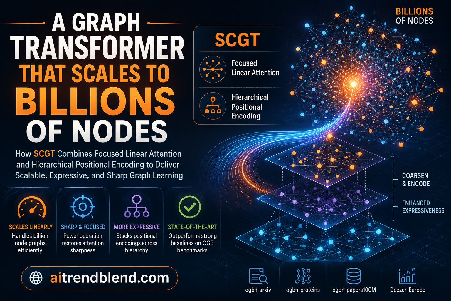
Transformers rewrote what was possible in language and vision, so pointing them at graphs looked like a sure bet. The bet mostly paid off on small graphs and mostly stalled on large ones. The reason is simple to state and hard to fix. Full attention compares every node with every other node, which costs the square of the number of nodes, and a graph with a hundred million nodes turns that quadratic cost into a wall. The usual escape, linear attention, makes the model fast but strangely dull, its attention spread so evenly that it can no longer tell important nodes from background. A team from Southeast University and Shanxi University asks whether you can have both, the speed of linear attention and the sharpness of full attention, on graphs with billions of nodes.
Key points
- Graph transformers shine on small graphs but their full attention scales with the square of the node count, which rules out large graphs.
- Linear attention fixes the cost but flattens the attention scores, so the model loses the ability to focus on the nodes that matter.
- SCGT introduces a focused linear attention that uses a power operation to sharpen the score distribution back toward what full attention would produce, while keeping linear cost.
- A comprehensive positional encoding stacks absolute and relative encodings across a coarsened graph hierarchy, so the model sees community and hierarchical structure it would otherwise miss.
- The authors prove the design is strictly more expressive than a standard distance based graph test, and show it beats strong baselines on twelve node classification datasets.
- SCGT scaled to a graph with more than a hundred million nodes and cut the time and memory of competitors by large margins on the biggest datasets.
Two problems that usually trade against each other
A graph transformer treats the nodes of a graph like tokens in a sentence and lets attention decide how much each node should listen to every other node. That global view is the appeal. Unlike a message passing network that only talks to immediate neighbors, attention can link two distant nodes directly, which sidesteps the well known troubles of message passing such as oversmoothing and oversquashing.
The appeal comes with a bill. Comparing all pairs of nodes costs \(O(n^2)\) in both time and memory, and the computation graph grows sharply as layers stack. In practice that has confined graph transformers to graphs with up to a few hundred nodes. On larger graphs they run out of memory, and in low data settings they tend to overfit and fall behind plain message passing networks. So the field went looking for cheaper attention.
Linear attention is the standard answer. It rewrites attention as a product of feature maps and uses the associativity of matrix multiplication to drop the cost from \(O(n^2)\) to \(O(n)\). The trick works, and methods like NodeFormer and SGFormer brought graph transformers to large graphs for the first time. But something is lost in the rewrite. The approximation produces a smooth attention distribution, one where scores are spread almost evenly across nodes. A model that attends to everything a little attends to nothing in particular, and that bluntness caps how expressive it can be.
There is a second, quieter problem. Graph transformers have weak inductive bias. A convolutional network knows about locality and a message passing network knows about the graph edges, but a transformer starts with no built in sense of graph structure. Researchers patch this with positional encodings, yet most encodings capture only pairwise distances and miss the larger picture. Real graphs are full of hierarchy. A protein molecule has functional groups nested inside it. Social and citation networks form communities with their own internal structure. Miss those and the model misses much of what the graph is about.
Focused attention, or how to sharpen without slowing down
The first half of SCGT is a mechanism the authors call focused graph linear attention, or FGLA. Its job is to recover the sharp, decisive score distribution of full attention while paying only linear cost. The idea is to bend each query and key vector so that similar pairs are pulled closer together and dissimilar pairs are pushed further apart before attention is computed.
The engine behind that bending is a focused function built on an element wise power operation. Each feature vector is raised to a power controlled by a factor the authors write as \(\alpha\), then rescaled so the operation preserves the length of the original vector. Raising to a power exaggerates the gap between a vector’s largest component and the rest, which is exactly what sharpens the eventual attention scores.
Read that in plain terms. A non negative activation \(\sigma\) makes the vector safe to work with, the power operation stretches the differences between its entries, and the rescaling by the original norm keeps the vector from growing or shrinking overall. Feed the focused queries and keys into linear attention and the associativity trick still applies, so the whole thing runs in linear time.
The authors back this with a proof rather than a hope. Their first proposition shows that for a suitable \(\alpha\) greater than one, the focused function makes similar query and key pairs score even higher and dissimilar pairs score even lower than raw attention would, which restores the sharp distinction that full attention gets from its exponential. In other words, the power operation is a cheap stand in for the expensive exponentiate step at the heart of standard attention.
FGLA adjusts the direction of each query vector and key vector, pulls similar pairs closer and pushes dissimilar pairs far away. Liang and colleagues, IEEE TPAMI 2026
The visual evidence is convincing. On molecular graphs from the ZINC dataset the authors plot attention scores for standard attention, for the linear method Performer, and for FGLA. Performer looks washed out. FGLA looks almost identical to full attention, concentrating on the chemically important atoms like nitrogen, sulfur, and chlorine that drive solubility. A node embedding plot on CiteSeer tells the same story, with FGLA producing tighter, more separable clusters than the linear baselines.
Positional encoding across a hierarchy
The second half of SCGT is about giving the transformer a real sense of structure. The authors call it comprehensive positional encoding, or CPE, and the core move is to compute positional information not just on the original graph but across a hierarchy of coarser versions of it.
To build that hierarchy they use graph coarsening, the same family of techniques that shrinks a large graph into a smaller one by merging groups of nodes into supernodes. Starting from the original graph they apply the METIS coarsening algorithm to produce a sequence of ever coarser graphs, each capturing structure at a broader scale. A mapping function records which original node lands in which supernode at every level, so information can be traced up and down the hierarchy.
On every level they compute two kinds of encoding. Absolute positional encoding, which records where a node sits, and relative positional encoding, which records how far apart pairs of nodes are. They then lift the encodings from each coarse level back to the size of the original graph and add them together, producing a hierarchical absolute encoding and a hierarchical relative encoding. The absolute part is added to the node features and the relative part becomes a bias inside the attention.
Why go to this trouble? Because pairwise distance on the original graph is a weak lens. The authors prove that their hierarchical relative encoding is strictly more expressive than shortest path distance under a standard graph distinguishing test called GD-WL, short for the generalized distance Weisfeiler-Leman test. They even exhibit two graphs, a Dodecahedron and a Desargues graph, that shortest path distance cannot tell apart but their encoding can. That is a concrete gain in the model’s ability to see structure, not just a claim.
SCGT also keeps a foot in the message passing world. The attention output is blended with the output of an ordinary graph neural network through a single mixing weight, so local neighborhood signal and global attention signal both contribute to the final representation.
Because the coarse graphs are so much smaller than the original, the bias terms and the coarsened encodings add only linear cost. The authors work through the accounting and land on an overall complexity of \(O(\lvert V \rvert + \lvert E \rvert)\), the node count plus the edge count. For the sparse graphs that dominate real applications, that is linear in the size of the graph, which is what makes the billion node claim credible.
How it performs
The evaluation spans twelve node classification datasets, split into seven medium sized graphs and five large ones. The medium set covers the familiar citation networks Cora, CiteSeer, and PubMed along with four heterophilic graphs including Actor, Squirrel, Chameleon, and Deezer-Europe. The large set climbs from ogbn-arxiv and ogbn-proteins through Amazon2M and pokec up to ogbn-papers100M, a graph with more than a hundred million nodes that sits near the top of public benchmarks.
On the medium graphs SCGT outperformed almost every recent strong baseline, both message passing networks and the newest graph transformers. On the large graphs the margin widened. The headline number is on the pokec social network, where SCGT reached 78.20 percent accuracy and cleared the second best model by a wide gap. Several competing transformers that look excellent on small graph tasks simply ran out of memory on these datasets.
| Dataset or test | Scale | Result for SCGT |
|---|---|---|
| ogbn-papers100M | More than 100 million nodes | Trained with decent efficiency where several transformers ran out of memory |
| pokec | Large social network | Reached 78.20 percent accuracy, well ahead of the second best model |
| Large datasets overall | Millions to billions of nodes | Cut competitor time by up to 90 percent and memory by up to 91.7 percent |
| Amazon2M scaling test | Growing node subsets | Scaled linearly while full attention ran out of memory near 60,000 nodes |
The scalability test makes the point crisply. On growing subsets of the Amazon2M graph, both time and memory for SCGT rose in a straight line with the number of nodes. The same model with full attention swapped back in hit an out of memory error once the subset passed roughly 60,000 nodes. Across the large datasets the authors report cutting the time cost of competing methods by as much as 90 percent and the memory cost by as much as 91.7 percent.
The ablation study confirms that each piece earns its place. Replacing focused attention with the plain linear method Performer hurt accuracy, and removing either the hierarchical absolute encoding or the hierarchical relative encoding hurt it too. A separate sweep of the focused factor found the best accuracy always landed at a value greater than one, across the whole range from one to ten, which lines up with the theory that the power operation is what sharpens the scores.
The honest limitations
The strong results come with real caveats. The first is tuning. SCGT carries a wide grid of hyperparameters, including the focused factor, the mixing weight between attention and the local network, the number of hierarchy levels, learning rate, hidden width, dropout, and the sizes of the coarse graphs. The authors ran a broad grid search to get their numbers. That search is a cost, and a practitioner adopting the method should expect to spend time on it rather than dropping it in unconfigured.
The second caveat is the reliance on coarsening quality. The whole comprehensive encoding rests on the hierarchy that graph coarsening produces, so the structure the model can see is only as good as the coarsening. The authors mostly use a single coarse level in their large scale runs, which limits how much hierarchy the model actually exploits, and coarsening a graph well is its own hard problem. If the coarsening merges the wrong nodes, the positional signal it feeds upward will be misleading.
Third, the evaluation is node classification from start to finish. The focused attention is demonstrated on molecular graphs for visualization, but the reported benchmarks are all node level prediction. Graph level tasks, link prediction, and other settings are left for future work, and the authors themselves flag robustness and broader applicability as open directions. The expressiveness proof is a real strength, yet it is a statement about distinguishing power under one particular test, not a guarantee of accuracy on every task.
None of this undercuts the contribution. It marks the edges of it. SCGT shows that the tradeoff between scalability and expressiveness is not as fixed as it looked, and it gives a concrete recipe for loosening it, while being honest that the recipe needs care to cook.
A reference implementation of focused attention
The heart of the method is compact enough to write directly. The code below implements the focused mapping, the focused linear attention, and a simplified SCGT block that adds a relative encoding bias and blends in a local graph network. A smoke test runs it on a small random graph. The original paper and the authors’ released code carry the full architecture and the hierarchy construction. Details are in the published IEEE TPAMI article.
# Focused Graph Linear Attention (FGLA) and a simplified SCGT block.
import torch
import torch.nn as nn
import torch.nn.functional as F


def focused_map(z, alpha, eps=1e-6):
    # Non negative activation, then an element wise power that sharpens
    # the vector while preserving its original norm.
    y = F.relu(z)
    y_pow = y ** alpha
    norm_y = y.norm(dim=-1, keepdim=True)
    norm_pow = y_pow.norm(dim=-1, keepdim=True).clamp(min=eps)
    return norm_y * y_pow / norm_pow


class FGLA(nn.Module):
    def __init__(self, dim, alpha=4.0):
        super().__init__()
        self.wq = nn.Linear(dim, dim, bias=False)
        self.wk = nn.Linear(dim, dim, bias=False)
        self.wv = nn.Linear(dim, dim, bias=False)
        self.alpha = alpha

    def forward(self, x, rel_bias=None):
        q = focused_map(self.wq(x), self.alpha)      # [n, d]
        k = focused_map(self.wk(x), self.alpha)      # [n, d]
        v = self.wv(x)                               # [n, d]
        # Linear attention via the associativity trick, cost O(n d^2).
        kv = k.transpose(-1, -2) @ v               # [d, d]
        num = q @ kv                                 # [n, d]
        den = (q @ k.sum(dim=0, keepdim=True).transpose(-1, -2))
        out = num / den.clamp(min=1e-6)
        if rel_bias is not None:
            # Relative encoding bias. The scalable model coarsens this term,
            # here we use the full n by n form for clarity.
            out = out + rel_bias @ v
        return out


def gcn_propagate(x, adj):
    # Symmetric normalized propagation, a plain message passing step.
    deg = adj.sum(dim=-1).clamp(min=1.0)
    dinv = deg.pow(-0.5)
    norm_adj = dinv.unsqueeze(1) * adj * dinv.unsqueeze(0)
    return norm_adj @ x


class SCGTBlock(nn.Module):
    def __init__(self, dim, ape_dim, alpha=4.0, beta=0.5):
        super().__init__()
        self.attn = FGLA(dim, alpha)
        self.ape_proj = nn.Linear(ape_dim, dim, bias=False)  # adds HAPE to features
        self.gnn = nn.Linear(dim, dim, bias=False)
        self.beta = beta

    def forward(self, x, adj, hape, hrpe):
        # Inject the hierarchical absolute encoding into the features.
        x_hat = x + self.ape_proj(hape)
        # Global focused attention with the hierarchical relative bias.
        x_attn = self.attn(x_hat, rel_bias=hrpe)
        # Blend global attention with a local message passing signal.
        x_local = self.gnn(gcn_propagate(x, adj))
        return (1.0 - self.beta) * x_attn + self.beta * x_local


def smoke_test():
    torch.manual_seed(0)
    n, d, s = 200, 32, 8
    x = torch.randn(n, d)
    # Random symmetric adjacency with a few edges per node.
    a = (torch.rand(n, n) < 0.03).float()
    adj = torch.triu(a, diagonal=1)
    adj = adj + adj.transpose(0, 1)
    hape = torch.randn(n, s)                 # stand in for merged absolute encoding
    hrpe = torch.softmax(torch.randn(n, n), dim=-1)  # stand in for relative bias

    block = SCGTBlock(dim=d, ape_dim=s, alpha=4.0, beta=0.5)
    out = block(x, adj, hape, hrpe)
    print(f"input {tuple(x.shape)}  output {tuple(out.shape)}")
    print(f"output mean {out.mean().item():.4f}  std {out.std().item():.4f}")


if __name__ == "__main__":
    smoke_test()
The version above uses the full relative bias matrix for readability, which is the one part that is not linear. In the real model that bias is transformed onto the small coarse graphs before it multiplies the values, which is exactly the step that keeps the whole block linear in the graph size. The focused mapping and the blend with a local network carry over directly.
Go to the source
Read the full paper, the proofs, and the twelve dataset results.
Read the paper IEEE XploreWhat this means for large graph learning
The lasting idea in SCGT is that the tradeoff between scalability and expressiveness was never a law of nature. It was a symptom of two specific shortcuts, flat attention scores and shallow positional encoding, and each shortcut has a fix that does not cost the speed you bought it for. Sharpen the scores with a norm preserving power operation, and enrich the encoding by looking at the graph across scales. Neither move reintroduces the quadratic cost, which is the whole point.
The focused attention idea travels beyond graphs. Any linear attention model that suffers from overly smooth scores, in language or vision as much as on graphs, could in principle borrow the same power operation to recover sharpness for close to nothing. The appeal of a fix that is a few lines of code and comes with a proof is that other architectures can test it quickly.
The hierarchy idea connects to a broader current in graph learning. Coarsening a graph to capture structure at multiple scales is the same instinct behind pooling in graph networks and behind fast methods that shrink graphs before processing them. SCGT uses coarsening not to save compute directly but to manufacture a richer positional signal, which is a fresh reason to care about coarsening quality and a nice link between two lines of work that often sit apart.
For a practitioner the practical read is encouraging with a footnote. If you have a very large graph and you want the global reach of attention without the memory explosion, SCGT is evidence that you can have it, with accuracy that beats strong baselines and cost that grows linearly. The footnote is the tuning. This is a method with many dials, and getting the reported results took a real search. Budget for that, lean on the released configurations as a starting point, and the payoff on graphs that used to be out of reach looks worth the effort.
More than any single benchmark, the value here is a reframing. Scalable and expressive were treated as opposites for graph transformers, and this work argues they are not, then backs the argument with proofs and results on graphs from thousands of nodes to more than a hundred million. That is the kind of result that changes what people attempt next.
Frequently asked questions
What is a graph transformer?
A graph transformer applies the attention mechanism from transformer models to the nodes of a graph, letting each node attend to others regardless of whether they are directly connected. This global view helps it capture long range relationships that message passing networks, which only talk to immediate neighbors, tend to miss.
Why do graph transformers struggle to scale?
Standard attention compares every pair of nodes, so its time and memory cost grows with the square of the number of nodes. On graphs with millions or billions of nodes that quadratic cost becomes impractical, which is why plain graph transformers have mostly been limited to small graphs.
What is focused graph linear attention?
It is the attention mechanism in SCGT that keeps the linear cost of efficient attention while restoring the sharp score distribution of full attention. It raises the query and key vectors to a power in a way that preserves their length, which pulls similar pairs closer and pushes dissimilar pairs apart so the model can focus on important nodes.
What does the comprehensive positional encoding add?
It gives the transformer a sense of structure at several scales. By coarsening the graph into a hierarchy and computing absolute and relative positional encodings on each level, then merging them, the model can see community and hierarchical structure. The authors prove this encoding is strictly more expressive than plain shortest path distance.
How large a graph can SCGT handle?
The authors ran it on ogbn-papers100M, a benchmark with more than a hundred million nodes, and report scaling to graphs with up to billions of nodes. Its overall cost grows with the number of nodes plus the number of edges, which is linear for the sparse graphs common in practice.
Where can I find the paper?
The work was published in IEEE Transactions on Pattern Analysis and Machine Intelligence in 2026 with DOI 10.1109/TPAMI.2026.3682858, by Jianqing Liang, Min Chen, Xinkai Wei, and Jiye Liang. The authors released code alongside the paper.
Source paper. Jianqing Liang, Min Chen, Xinkai Wei, and Jiye Liang, SCGT, Toward Scalable and Comprehensive Graph Transformer, IEEE Transactions on Pattern Analysis and Machine Intelligence, volume 48, number 8, August 2026, pages 9312 to 9322. DOI 10.1109/TPAMI.2026.3682858.
This analysis is based on the published paper and an independent evaluation of its claims.