
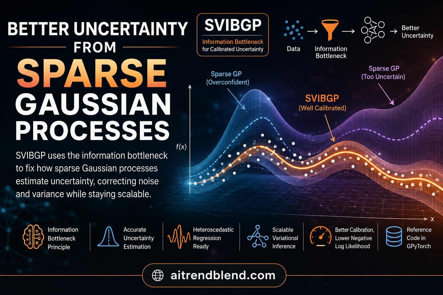
A regression model tells you it is very confident, and it is wrong. That failure is more dangerous than a wrong answer with an honest wide error bar, because a confident mistake gives you nothing to hedge against. Gaussian processes were supposed to solve exactly this. They carry a full distribution over functions and hand back calibrated uncertainty for free. So why do the fast, scalable versions of them so often report the wrong amount of doubt?
Key points
- Sparse Gaussian processes trade exact inference for speed, and that trade quietly damages their uncertainty estimates in two opposite ways.
- The standard sparse method SVGP overstates the observation noise and barely uses input dependent variance, so it cannot model data whose noise changes across the input space.
- The competing method PPGPR fixes point wise sharpness but drives observation noise toward zero, which produces an ill conditioned predictive covariance and unstable joint predictions.
- Liang Mao and Shiliang Sun show both methods are optimizing a lower bound on the same information bottleneck objective, each in a flawed way.
- Their fix, SVIBGP, splits the mutual information into two parts and uses two coupled decoders with a stop gradient trick, so the model captures changing noise without underestimating the base noise.
- Across seven regression datasets SVIBGP kept the low negative log likelihood of PPGPR while avoiding its exploding predictive density, at a compute cost close to the older methods.
Where sparse Gaussian processes lose the plot
A Gaussian process is a beautiful object. It places a prior over functions, conditions on data, and returns a posterior that says both what it predicts and how sure it is. The catch is cost. Exact inference scales with the cube of the number of data points, written \(O(N^3)\), which stops being practical somewhere in the tens of thousands of samples. Real datasets are much larger than that.
The standard escape is to summarize the process with a small set of \(M\) inducing points, which drops the cost to \(O(NM^2)\). Combine that with stochastic optimization over minibatches and you get the sparse variational Gaussian process, or SVGP, which scales to big data. This is the workhorse that put Gaussian processes back on the table for large problems.
Here is where it gets interesting. SVGP buys its speed with an approximation, and the approximation has a personality. It tends to blame everything on noise. When the model sees scatter in the data, it attributes most of that scatter to input independent observation noise, the term \(\sigma^2_{obs}\), rather than to the input dependent variance of the latent function, \(\sigma^2_x\). The consequence is that SVGP produces a nearly flat uncertainty band. It cannot say that predictions are shaky in one region and solid in another, because it never learned to let the function variance do that work.
That property has a name. Data whose noise level changes across the input space is called heteroscedastic, and it is everywhere in the real world. Sensor readings get noisier under load. Financial signals get noisier in a crisis. A model that assumes one constant noise level across the whole input space, which is what SVGP effectively falls back to, will be overconfident where the data is messy and underconfident where it is clean.
The first fix, and its new problem
An earlier method called the parametric predictive Gaussian process regressor, or PPGPR, spotted this and offered a repair. Its diagnosis was sharp. The metric people use to judge uncertainty is the log predictive density, which includes the posterior variance in its data fitting term. The training objective of SVGP, the evidence lower bound, uses only the observation noise in that spot and leaves the posterior variance out. Train on one thing, grade on another, and you should not be surprised when the grades disappoint.
PPGPR closes that gap by treating the predictive density itself as the thing to fit, then doing a regularized maximum likelihood estimation on it. The move works for point wise calibration. PPGPR produces excellent sharp uncertainties, and on the negative log likelihood metric it looks superb.
But the cure introduces a new disease. PPGPR tends to push the observation noise \(\sigma^2_{obs}\) toward zero. In the predictive density the observation noise and the function variance appear symmetrically, so the model cannot tell them apart from the log likelihood alone, and it collapses the noise term to sharpen its score. Once \(\sigma^2_{obs}\) is nearly zero the predictive covariance becomes ill conditioned. Its condition number blows up, the joint predictive distribution over a test set turns nearly singular, and the negative log predictive density on that test set explodes.
There is a subtle warning buried in this comparison, and the authors draw it out. The negative log likelihood, the very metric PPGPR optimizes so well, is a flawed judge on its own. Because it rewards alignment between predicted uncertainty and error, a model with large errors but large stated uncertainty can still post a good score. A method can look excellent on negative log likelihood while being worse on plain root mean squared error than a simpler baseline. Any single uncertainty metric can be gamed, which is why the paper reports four of them side by side.
Reframing the problem through information theory
The contribution of Mao and Sun is to stop treating these as two unrelated tricks and to show they are both special cases of one principle. That principle is the information bottleneck, an idea from information theory that asks a learner to compress its input while keeping whatever is relevant to the target. Formally you maximize the information a representation carries about the label while penalizing the information it carries about the input.
Read the two terms as a pull and a push. The first term pulls the representation \(t_x\) toward being useful for predicting \(y\). The second term, weighted by \(\beta\), pushes it toward forgetting the raw input, which is compression. The authors take the latent function value at a point as the representation and show, with two theorems, that both SVGP and PPGPR are maximizing a lower bound of this exact objective.
The trouble is how each one does it. SVGP applies the bottleneck in what the authors call a coarse grained manner. Its representation carries a mean and a variance, but the objective effectively ignores one branch, the variance, and lets the model focus on the mean alone. Information about the target that lives in the variance simply never enters the bound, and once lost it cannot be recovered later. PPGPR does use both mean and variance, but it picks a decoder that is not identifiable, meaning two different noise splits look identical to it, and it has no direct handle on the compression term. That is the formal reason it cannot keep the observation noise honest.
Following the guidance of the IB theory, we arrive at a natural and effective solution. Mao and Sun, IEEE TPAMI 2026
Seeing both methods as bounds on one objective is more than tidy bookkeeping. It tells you where to intervene. If the problem is that one branch of information gets dropped and the other gets no compression control, then the fix is to handle the two branches separately and give the compression term something to grip.
The SVIBGP solution
The method the authors propose is the sparse variational information bottleneck Gaussian process, or SVIBGP. The core move is a decomposition. Rather than bounding the mutual information between the target and the pair of mean and variance all at once, they split it into two pieces using the chain rule. One piece is the information the mean carries about the target. The other is the extra information the variance carries once the mean is known.
Each piece gets its own decoder, and the design of the two decoders is the clever part. The first decoder reconstructs the target from the mean alone and uses only the observation noise, so its whole job is to set a sensible base noise level that explains the errors of the mean. The second decoder brings in the function variance and asks it to explain the leftover, the heteroscedastic structure that a single constant noise cannot capture.
Notice the hat on the mean in the second decoder. That is a stop gradient. In practice the authors block the gradient from flowing into the mean through this second term, so the mean is treated as a fixed reference there. Without that block the two decoders fight over the mean and, in the weakly regularized regime that these models prefer, the second decoder can overfit. With the block, the function variance is forced to earn its keep by explaining the residual rather than quietly reshaping the mean. It is a small implementation detail with a real effect on calibration.
Putting the two data fitting terms together with the usual regularizer on the inducing variables gives the training objective. The regularizer is the Kullback-Leibler divergence between the variational distribution over the inducing variables and their prior, scaled by \(\beta\) and the dataset size.
The path from analysis to method is unusually direct here. The information theory read told the authors precisely what was broken, one branch ignored and one decoder non identifiable, and the two decoder design addresses each fault in turn. This is the kind of result where the theory is not decoration bolted onto an empirical trick. The theory is the reason the trick has the shape it does.
Does it hold up on data
The synthetic test is the cleanest illustration. The authors build a one dimensional regression task with a fixed background noise of variance 0.49 plus a heteroscedastic component that drops to zero in places. Because the ground truth noise is known, you can see exactly who gets it right. SVGP behaves like an exact Gaussian process and misses the heteroscedasticity entirely, its uncertainty dominated by observation noise. PPGPR crushes the observation noise so hard that its predictive variance is nearly identical to the posterior variance. SVIBGP lands where a model with the true noise fixed in place would land, which is the target behavior.
On real data the story sharpens. Across seven regression datasets the authors compare eleven methods, including decoupled variants and several recent sparse approximations, using four metrics. The pattern is consistent. PPGPR and its decoupled version win the negative log likelihood but post exceptionally high negative log predictive density, the exploding covariance problem showing up on the test set. SVIBGP holds the lowest negative log likelihood among the well behaved methods while keeping its predictive density competitive or better.
| Method | Observation noise | Heteroscedasticity | Predictive stability |
|---|---|---|---|
| SVGP | Overestimated | Largely missed | Stable but flat |
| PPGPR | Driven near zero | Captured | Ill conditioned, high NLPD |
| SVIBGP | Kept close to truth | Captured | Stable, low NLPD and NLL |
Two more results matter for anyone deciding whether to adopt this. First, SVIBGP reached the best or second best root mean squared error on all seven datasets, so the improved calibration did not come at the price of worse point predictions, which is often the fear. Second, the training cost sits close to PPGPR and SVGP. The overhead is a single extra data fitting term, and the overall complexity is \(O(M^3 + BM^2)\) with \(B\) the minibatch size. You are not paying a large tax for the better uncertainty.
The calibration plots make the behavior tangible. Binning test points by predicted variance and plotting mean squared error against predicted variance, a well calibrated model should follow the diagonal. On a homoscedastic dataset where an exact Gaussian process aligns perfectly, both SVGP and SVIBGP shift right because they overestimate the noise, but SVIBGP shifts far less. On datasets with real heteroscedastic structure, the models that assume constant noise fail to track the fluctuating error, while SVIBGP and PPGPR follow the ideal line more closely. SVIBGP gets the honest middle ground, conservative enough to avoid PPGPR overfitting yet responsive enough to model the changing noise.
The honest limitations
No method escapes tradeoffs, and this paper is candid about several. The stop gradient helps most in the weakly regularized regime, when \(\beta\) is small, which happens to be where SVIBGP performs best. As \(\beta\) grows the benefit of the stop gradient fades and the two variants converge. So the trick is not a universal free lunch. It buys the most in exactly the setting the method favors, and a practitioner running with a large \(\beta\) will see less from it.
Choosing \(\beta\) is itself a tuning burden. The authors find SVIBGP prefers small values, with the sweet spot between 0.01 and 1, and performance falling off once \(\beta\) climbs above 1. They suggest treating the set 0.01, 0.1, and 1 as candidates. That is a manageable search, but it is a search, and it means the method is not entirely hands off.
The authors also explored an alternative regularizer that directly controls the compression term, derived cleanly from the theory. In practice it demanded strong regularization and careful tuning of one or two extra hyperparameters, and because of the symmetry between the noise and the function variance it could tip the model back into overestimating observation noise. They judged the payoff not worth the added tuning and set it aside. That is a useful negative result to report rather than hide, since it marks a path that looks promising on paper but costs more than it returns.
Finally, the evaluation lives entirely on regression with Gaussian likelihoods. The information bottleneck framing is general, and the authors position the work as one more way to train Gaussian processes with an objective other than the evidence lower bound, but classification and non Gaussian likelihoods are left for future work. The claims are strong within regression and should not be stretched past it without checking.
A reference implementation in GPyTorch
The method is built on GPyTorch, and the essential idea fits in a compact model plus a custom loss. The code below defines a sparse variational Gaussian process, then implements the SVIBGP objective with its two coupled decoders and the stop gradient on the mean. A training loop and a smoke test on synthetic heteroscedastic data round it out. The original paper and its supplementary material are available through the published IEEE TPAMI article.
# SVIBGP reference implementation on top of GPyTorch.
# Two coupled decoders with a stop gradient on the mean.
import math
import torch
import gpytorch
from gpytorch.models import ApproximateGP
from gpytorch.variational import CholeskyVariationalDistribution, VariationalStrategy
from gpytorch.means import ConstantMean
from gpytorch.kernels import ScaleKernel, RBFKernel
from gpytorch.likelihoods import GaussianLikelihood
from gpytorch.distributions import MultivariateNormal


class SVIBGP(ApproximateGP):
    def __init__(self, inducing_points):
        m = inducing_points.size(0)
        var_dist = CholeskyVariationalDistribution(m)
        var_strat = VariationalStrategy(
            self, inducing_points, var_dist, learn_inducing_locations=True
        )
        super().__init__(var_strat)
        self.mean_module = ConstantMean()
        # RBF kernel with one length scale per input dimension.
        self.covar_module = ScaleKernel(RBFKernel(ard_num_dims=inducing_points.size(1)))

    def forward(self, x):
        mean_x = self.mean_module(x)
        covar_x = self.covar_module(x)
        return MultivariateNormal(mean_x, covar_x)


def gaussian_logpdf(y, mean, var):
    # Elementwise Gaussian log density with variance var.
    return -0.5 * (((y - mean) ** 2) / var + torch.log(2.0 * math.pi * var))


def svibgp_loss(model, likelihood, x, y, num_data, beta=1.0, stop_gradient=True):
    # Latent posterior q(f_x) at the batch inputs.
    f_dist = model(x)
    mu = f_dist.mean                          # mean of the latent function
    var = f_dist.variance                     # input dependent latent variance
    sigma_obs2 = likelihood.noise             # observation noise, a learned scalar

    # Decoder 1: reconstruct y from the mean, using only observation noise.
    # This term sets an honest base noise level for the mean errors.
    term1 = gaussian_logpdf(y, mu, sigma_obs2)

    # Decoder 2: bring in the function variance to explain the residual.
    # Stop the gradient on the mean so var is forced to do this work.
    mu_ref = mu.detach() if stop_gradient else mu
    total_var = var + sigma_obs2
    term2 = gaussian_logpdf(y, mu_ref, total_var)

    # Minibatch estimate of the full data fitting integral.
    batch = x.size(0)
    data_fit = (num_data / batch) * (term1 + term2).sum()

    # Regularizer on the inducing variables, KL[q(f_Z) || p(f_Z)].
    kl = model.variational_strategy.kl_divergence().sum()

    objective = data_fit - beta * kl
    return -objective / num_data                # minimize the negative objective


def train(model, likelihood, x, y, steps=300, beta=0.1, lr=0.01):
    model.train()
    likelihood.train()
    params = list(model.parameters()) + list(likelihood.parameters())
    opt = torch.optim.Adam(params, lr=lr)
    n = x.size(0)
    for step in range(steps):
        opt.zero_grad()
        loss = svibgp_loss(model, likelihood, x, y, num_data=n, beta=beta)
        loss.backward()
        opt.step()
        if step % 50 == 0:
            print(f"step {step:4d}  loss {loss.item():.4f}  "
                  f"obs_noise {likelihood.noise.item():.4f}")


def evaluate(model, likelihood, x):
    # Return predictive mean and total predictive variance at x.
    model.eval()
    likelihood.eval()
    with torch.no_grad(), gpytorch.settings.fast_pred_var():
        f = model(x)
        mean = f.mean
        total_var = f.variance + likelihood.noise
    return mean, total_var


def smoke_test():
    torch.manual_seed(0)
    # Synthetic heteroscedastic data. Base noise 0.49 plus a noise
    # component that grows with x, matching the paper's setup.
    x = torch.linspace(-3.0, 3.0, 400).unsqueeze(-1)
    clean = torch.sin(x)
    hetero = 0.3 * torch.clamp(x, min=0.0) * torch.randn_like(x)
    base = math.sqrt(0.49) * torch.randn_like(x)
    y = (clean + base + hetero).squeeze(-1)

    inducing = torch.linspace(-3.0, 3.0, 20).unsqueeze(-1)
    model = SVIBGP(inducing)
    likelihood = GaussianLikelihood()

    train(model, likelihood, x, y, steps=300, beta=0.1)
    mean, total_var = evaluate(model, likelihood, x)
    print(f"final obs noise {likelihood.noise.item():.4f}  "
          f"mean pred var {total_var.mean().item():.4f}")


if __name__ == "__main__":
    smoke_test()
The version above is written for clarity rather than for a benchmark. A real run would use minibatches through a data loader, hold out a validation split to pick \(\beta\), and evaluate the negative log predictive density on the joint test distribution rather than the per point density. The key logic to carry over is the two term data fit and the detach on the mean in the second term, since that stop gradient is what keeps the observation noise honest.
Go to the source
Read the full paper and the derivations behind the two decoder design.
Read the paper GPyTorch libraryWhat this means for practitioners
Step back and the lesson is broader than one model. For years the community treated poor Gaussian process uncertainty as a bag of separate quirks, one method too timid, another too bold, each patched with its own heuristic. Reading the two failures as different corners of a single information bottleneck objective turns a pile of fixes into one diagnosis. That reframing is the real contribution, and it is the sort of move that tends to keep paying off, because the next uncertainty method can be checked against the same yardstick rather than judged by vibes.
The practical payoff is a model you can trust to say when it does not know. In any setting where a wrong prediction carries asymmetric cost, an active learning loop deciding what to sample next, a controller deciding when to defer to a human, a forecast feeding a downstream decision, the width of the error bar is not a nicety. It is the signal you act on. A method that keeps the base noise honest while still widening where the data is genuinely noisy gives that signal a fair chance of being right.
The idea also travels. The information bottleneck view is not tied to Gaussian processes, and the coupled decoder decomposition is a general recipe for any model that reports a mean and a variance and struggles to keep the two from stepping on each other. The stop gradient is a portable trick. Anyone building calibrated regressors, from neural networks with predicted variance heads to other probabilistic models, can borrow the pattern of forcing the variance to explain the residual rather than reshaping the mean.
The honest edges remain. The method wants a small compression weight to shine, the choice of that weight needs a short search, and everything so far is regression with Gaussian noise. None of that undercuts the core result. It maps the frontier. The obvious next steps are classification, non Gaussian likelihoods, and a deeper look at whether the coupled decoder idea improves calibration in large neural models too. Those are extensions, not repairs.
For now the takeaway is clean. If you use sparse Gaussian processes and you care about the uncertainty and not just the mean, the default methods are quietly failing you in one of two directions, and there is a principled way to stop both failures at once without giving up scalability. When the uncertainty is the product, that is the result that matters.
Frequently asked questions
What is a sparse variational Gaussian process?
It is a scalable approximation to a Gaussian process that summarizes the full dataset with a small set of inducing points and uses variational inference to fit them. This drops the cost from growing with the cube of the number of data points to something that scales with the inducing points and the minibatch size, which lets Gaussian processes handle large datasets.
Why do sparse Gaussian processes give poor uncertainty?
The approximation biases where variance gets attributed. The standard method SVGP tends to blame most scatter on constant observation noise and ignores the input dependent function variance, so it cannot model data whose noise changes across the input. The competing method PPGPR overcorrects and drives observation noise toward zero, which makes the predictive covariance unstable.
What is the information bottleneck principle?
It is an idea from information theory that asks a model to compress its input while keeping the information relevant to the target. You maximize how much the learned representation tells you about the label while penalizing how much it retains about the raw input, which yields a representation that is useful and robust to noise.
How does SVIBGP fix the uncertainty problem?
SVIBGP splits the mutual information between the target and the model output into two parts, one for the mean and one for the variance, and gives each its own decoder. The first decoder sets an honest base noise level from the mean errors, and the second uses the function variance to explain the leftover heteroscedastic structure, with a stop gradient so the variance cannot quietly reshape the mean.
Is SVIBGP slower than existing methods?
Not by much. The extra cost is one additional data fitting term, so the training and testing time stay close to SVGP and PPGPR. The overall computational complexity is on the order of the cube of the inducing point count plus the minibatch size times the square of that count.
Where can I find the paper and the tools?
The work was published in IEEE Transactions on Pattern Analysis and Machine Intelligence in 2026 with DOI 10.1109/TPAMI.2026.3675000, by Liang Mao and Shiliang Sun. The method is implemented with GPyTorch, an open source Gaussian process library for PyTorch.