
Key points
- The work compresses large scientific measurements by fitting a small neural network to them, an approach called an implicit neural representation.
- Small networks suffer from spectral bias, meaning they learn low frequency structure easily and struggle with the high frequency detail that carries much of the physics.
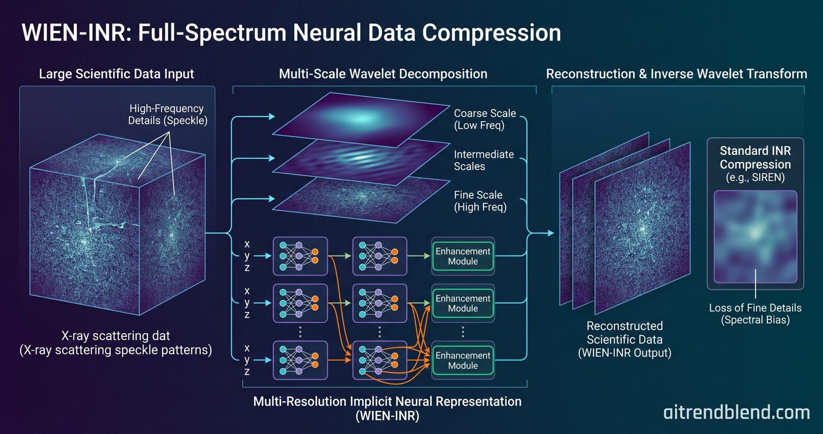
- WIEN-INR splits the signal into wavelet frequency bands and fits a dedicated small network to each, then adds an enhancement module that recovers the finest details without inflating the model.
- On a Cu3Au X-ray scattering volume it reached 43.6 decibels and a structural similarity of 0.97 at about 30 times smaller than the raw data, the best of every method tested.
- It preserves the speckle contrast that scattering physics depends on, holding about 95 percent of it, where competing networks wash it out.
- A theoretical result shows the band split design is provably as good as or better than a single monolithic network at capturing high frequency content under a fixed parameter budget.
Why store data as a network at all
The idea underneath this work sounds strange the first time you hear it. Instead of saving a measurement as the array of numbers it obviously is, you train a neural network to output the value at any coordinate you ask for, then throw the original array away and keep only the network. Ask the trained network for the intensity at a given detector pixel and it computes the answer. The data has become a function.
These are called implicit neural representations, and they have a genuinely useful property. The size of the stored network depends on how complex the signal is, not on how many voxels the original grid had. Double the resolution of your detector and a voxel file doubles in size, but a neural representation of a signal with the same underlying structure barely grows. The representation is also continuous and differentiable, so you can query it at any resolution, take gradients, and decode just a region of interest without unpacking the whole thing. For scientific pipelines drowning in measurement data, that is an appealing set of features.
There is a well known problem, though, and it is the reason naive versions of this idea disappoint. A small neural network trained to fit a signal does not treat all frequencies equally. It races to capture the smooth, low frequency trends and drags its feet on the high frequency detail, the sharp edges and fine textures. Researchers call this spectral bias, and it is not a bug you can tune away easily. It is baked into how gradient descent fits a coordinate network. For a photograph you might not care. For a scattering measurement, where the fine speckle pattern is the signal you came to measure, losing the high frequencies means losing the science.
Splitting the signal by frequency
Yuan Ni and colleagues attack the spectral bias at its root by refusing to make one network do everything. Their method, WIEN-INR, first passes the data through a wavelet transform. If you have not met wavelets, the short version is that they decompose a signal into components at different scales, separating the broad low frequency trends from the localized high frequency details, and doing so in a way that keeps track of where in the signal each detail lives. Unlike a Fourier transform, which spreads a sharp edge across every frequency, a wavelet transform keeps a sharp edge local, which is exactly right for the transient and localized features common in scientific data.
Once the signal is split into these frequency bands, WIEN-INR fits a separate small network to each band. The coarse bands, which hold smooth low frequency content, get small networks because they do not need much capacity. The fine bands, which hold the detail, get more. This is the first half of the idea, and it already helps, because each network only has to represent one slice of the frequency spectrum rather than fighting the spectral bias across the whole range at once. The authors call this baseline WAVELET-INR.
The training objective is simply to match the wavelet coefficients of the signal at each scale.
Here \(\varphi_{\omega_j}\) is the small network for scale \(j\) and \(\mathbf{d}_j\) are the true wavelet detail coefficients at that scale. Because the wavelet transform is an orthonormal operation, matching the coefficients is equivalent to matching the reconstructed signal, so this decomposition costs nothing in fidelity while making each network’s job far easier.
The enhancement module that recovers the finest detail
Splitting by frequency helps, but the very finest band, the one holding the sharpest textures, remains hard for a small network to represent. This is where the paper’s central contribution comes in, an enhancement module that boosts a network’s ability to capture fine detail without making it much bigger.
The mechanism is a coarse to fine refinement. The module takes the prediction at a coarser scale, upsamples it to serve as a geometric guide to where the finer detail should live, and then a lightweight learnable network predicts the finer coefficients conditioned on that guide. In effect it learns a local operator that says, given how the signal looks at this coarser resolution, here is how the next finer scale should sharpen it. Because the guide already carries most of the structure, the refinement network only has to learn the correction, which is a much smaller job than learning the finest band from scratch.
Adding this module turns WAVELET-INR into WIEN-INR, and the gap between them is the whole argument. Same wavelet split, same coarse networks, but with a small enhancement network aimed at the finest details, the reconstruction of high frequency texture improves sharply while the total model size barely moves. The authors are careful to note the module is standalone. It is not welded to one architecture, and it can be bolted onto any coordinate based representation.
The enhancement module infers finer scale details conditioned on coarser scale estimations, effectively acting as a learnable local operator that enhances the ability of the network to capture the finest details. Ni and colleagues, on the module at the heart of WIEN-INR
A theory that says splitting is the right move
What lifts this above a clever engineering trick is that the authors prove the split is not just convenient but optimal in a precise sense. Working in a regime where wide networks behave like a fixed kernel, described by the neural tangent kernel, they analyze how a fixed parameter budget should be spent to capture high frequency content to a target accuracy.
Their main theorem states that splitting the network across frequency bands, which gives the kernel a block structure, is capacity optimal at a fixed high frequency target. Put plainly, for a given number of parameters, a network that dedicates separate blocks to separate bands captures the high frequencies at least as well as, and generally better than, a single monolithic network of the same size trying to do everything at once.
The term on the left is the parameters a band split network needs to hit a high frequency error target, and the term on the right is what a monolithic network needs. The split never needs more, and usually needs fewer. It is a satisfying result because it turns a design intuition, give each frequency its own machinery, into a statement you can prove under stated assumptions rather than just observe.
What the benchmarks show
The authors test on a demanding spread of real experimental data, six scientific datasets covering wide angle coherent X-ray scattering from the intermetallic alloy Cu3Au, four dimensional inelastic neutron scattering, ultrafast X-ray scattering from a free electron laser, coherent diffraction imaging, ptychography, and solar magnetogram data from a space telescope. These are not toy images. They span vastly different scales, physics, and structure, which is the point, since the claim is about full spectrum fidelity across modalities.
On the Cu3Au scattering volume, WIEN-INR reached 43.6 decibels of peak signal to noise ratio and a structural similarity of 0.97 while compressing the data to about 30 times smaller than the raw array. That was the best of every method compared, a field that included the strong coordinate network families SIREN, WIRE, FINER, and MINER, along with hash encoding and Fourier feature approaches. On pixelwise consistency across the full volume it reached the highest score of any method, and crucially it retained about 95 percent of the speckle contrast, the statistical fingerprint that downstream scattering analysis actually reads.
| Aspect | WIEN-INR result | Why it matters |
|---|---|---|
| Cu3Au scattering fidelity | 43.6 dB, 0.97 similarity, 1.33 MB | Best of all methods, about 30 times smaller than raw |
| Speckle contrast retained | About 95 percent | Preserves the statistical signal scattering analysis depends on |
| Local error at Bragg peaks | 2 to 7 times smaller | Fidelity where the physics is concentrated, not just on average |
| Decoding throughput | About 848 million voxels per second | Fast region of interest readout at roughly 13 milliseconds |
Two results matter more than the headline number. First, the local error. Averaged fidelity can hide failures that cluster exactly where you care, so the authors measured error around the Bragg peaks and the weak diffuse scattering regions specifically, and WIEN-INR cut it by two to seven times against the baselines. Competing networks tended to either over smooth the fine structure or invent unphysical textures, both of which are worse than they sound when a physicist is about to draw conclusions from the reconstruction. Second, the reconstruction tasks. For coherent diffraction imaging and ptychography, where the stored data has to be run back through a numerical solver to recover a real space image, WIEN-INR kept sharp edges and detail that the strong baseline SIREN smeared, compressing a 625 megabyte ptychography measurement to under 15 megabytes while preserving the reconstruction.
On speed, the practical concern with these representations is that they are slow to encode, since encoding means training a network. WIEN-INR helps here too, because splitting the training across wavelet scales yields smaller and easier learning problems per band, several of which can run in parallel. Within the same training time budget it reached the highest fidelity of any method tested, and decoding is nearly instant, needing only a network evaluation and an inverse wavelet transform.
Honest limitations
The authors are clear about where the method gives less. The gains are largest on data with rich fine scale structure, the speckle heavy scattering measurements where the finest band carries real information. On smooth natural images the picture inverts. There the multiscale machinery is overhead that does not pay for itself, and the average fidelity gains are modest and can even shrink at low bit rates, though the visual quality near sharp edges still improves. This is a method built for a particular kind of data, and it does not pretend otherwise.
Encoding speed is the persistent weakness of the whole family, not just this method. Fitting a neural representation means training, and training is slow compared to a conventional compressor that just runs an algorithm. WIEN-INR narrows the gap by splitting the work into smaller parallel problems, but it does not close it, and for workflows that need instant compression this remains a real constraint. The one place the parallelism breaks down is the finest scale, because the enhancement module there depends on the output of the next coarser network, so that final refinement cannot be fully parallelized.
There are smaller caveats worth naming. The storage saving relies on a simple reduction of the weights to half precision, and the authors point to more sophisticated compression of the network itself as future work rather than something already done. The theory that motivates the design holds in an idealized wide network regime and assumes a parameter budget rather than accounting for the finite training time that shapes real spectral bias, a gap the authors flag explicitly. None of this undercuts the results, but it marks the edges of where the guarantees apply.
Reproducing the enhancement idea
The core of WIEN-INR is a set of small coordinate networks fitting wavelet bands, plus an enhancement network that refines the finest band using a coarser prediction as a guide. The implementation below writes exactly that. It builds sine activation networks, splits a target with a Haar wavelet transform, fits the bands, and compares reconstruction quality with and without the enhancement module on the finest band. A runnable smoke test on a texture rich target shows the enhancement lifting the reconstruction by a wide margin, the same effect the paper reports between WAVELET-INR and WIEN-INR.
# Wavelet neural representation with a coarse-to-fine enhancement module.
# Educational reimplementation of the idea behind WIEN-INR from Ni,
# Chen, et al., "Multi-resolution enhancement for full-spectrum neural
# representations" (Nature Machine Intelligence 2026). One wavelet level
# and a single enhanced finest band, enough to show the mechanism.

import torch
import torch.nn as nn
import math


class Sine(nn.Module):
    """Sine activation, the SIREN nonlinearity."""
    def __init__(self, w0=30.0):
        super().__init__()
        self.w0 = w0

    def forward(self, x):
        return torch.sin(self.w0 * x)


class SIREN(nn.Module):
    """Coordinate MLP with sine activations and the SIREN init scheme."""
    def __init__(self, inp=2, out=1, hidden=64, layers=3, w0=30.0):
        super().__init__()
        net = [nn.Linear(inp, hidden), Sine(w0)]
        for _ in range(layers - 1):
            net += [nn.Linear(hidden, hidden), Sine(w0)]
        net += [nn.Linear(hidden, out)]
        self.net = nn.Sequential(*net)
        with torch.no_grad():
            self.net[0].weight.uniform_(-1 / inp, 1 / inp)
            for m in self.net[2::2]:
                if isinstance(m, nn.Linear):
                    b = math.sqrt(6 / hidden) / w0
                    m.weight.uniform_(-b, b)

    def forward(self, x):
        return self.net(x)


def haar_dwt2(img):
    """One level Haar wavelet transform. Returns LL, LH, HL, HH bands."""
    a, b = img[0::2, 0::2], img[0::2, 1::2]
    c, d = img[1::2, 0::2], img[1::2, 1::2]
    return (a + b + c + d) / 2, (a - b + c - d) / 2, \
           (a + b - c - d) / 2, (a - b - c + d) / 2


def haar_idwt2(LL, LH, HL, HH):
    """Inverse Haar transform, stitching the four bands back together."""
    H2, W2 = LL.shape
    out = torch.zeros(H2 * 2, W2 * 2)
    out[0::2, 0::2] = (LL + LH + HL + HH) / 2
    out[0::2, 1::2] = (LL - LH + HL - HH) / 2
    out[1::2, 0::2] = (LL + LH - HL - HH) / 2
    out[1::2, 1::2] = (LL - LH - HL + HH) / 2
    return out


def grid(H, W):
    """Normalized coordinate grid in the range minus one to one."""
    ys = torch.linspace(-1, 1, H)
    xs = torch.linspace(-1, 1, W)
    gy, gx = torch.meshgrid(ys, xs, indexing="ij")
    return torch.stack([gx.flatten(), gy.flatten()], 1)


def psnr(a, b):
    """Peak signal to noise ratio in decibels."""
    mse = ((a - b) ** 2).mean()
    rng = (b.max() - b.min()).clamp(min=1e-6)
    return (20 * torch.log10(rng) - 10 * torch.log10(mse)).item()


def texture_target(H, W, seed):
    """A smooth base plus structured high frequency texture."""
    torch.manual_seed(seed)
    g = grid(H, W)
    X = g[:, 0].reshape(H, W)
    Y = g[:, 1].reshape(H, W)
    smooth = torch.exp(-(X ** 2 + Y ** 2) * 2)
    tex = 0.0
    for fx, fy, ph in [(9, 7, 0.0), (13, 11, 0.7), (17, 5, 1.3),
                       (6, 15, 2.1), (19, 9, 0.4), (11, 17, 1.8)]:
        tex = tex + torch.sin(fx * math.pi * X + ph) * torch.sin(fy * math.pi * Y - ph)
    return smooth + 0.30 * tex


def fit_representation(img, use_enhancement, epochs=900,
                       hid_coarse=64, hid_fine=8, lr=1e-3):
    """Fit wavelet bands with small SIRENs, optionally enhancing HH.

    The coarse network fits the approximation and the two coarse detail
    bands. A deliberately tiny network fits the finest band HH. With
    enhancement, an extra network refines HH using the coarse prediction
    as a geometric guide, the WIEN-INR idea. Returns reconstruction PSNR.
    """
    H, W = img.shape
    LL, LH, HL, HH = haar_dwt2(img)
    coords = grid(H // 2, W // 2)

    coarse = SIREN(2, 3, hid_coarse, 3)     # fits LL, LH, HL
    fine = SIREN(2, 1, hid_fine, 2)        # small base for HH
    models = [coarse, fine]
    enhancer = None
    if use_enhancement:
        enhancer = SIREN(3, 1, 20, 3)         # coords plus coarse guide
        models.append(enhancer)

    params = [p for m in models for p in m.parameters()]
    opt = torch.optim.Adam(params, lr=lr)
    LLf, LHf, HLf, HHf = LL.flatten(), LH.flatten(), HL.flatten(), HH.flatten()

    for _ in range(epochs):
        opt.zero_grad()
        oc = coarse(coords)                       # [N, 3]
        loss = ((oc[:, 0] - LLf) ** 2).mean() \
             + ((oc[:, 1] - LHf) ** 2).mean() \
             + ((oc[:, 2] - HLf) ** 2).mean()
        hh_pred = fine(coords).squeeze(-1)
        if enhancer is not None:
            guide = oc[:, 0:1].detach()            # coarse LL as guide
            hh_pred = hh_pred + enhancer(torch.cat([coords, guide], 1)).squeeze(-1)
        loss = loss + ((hh_pred - HHf) ** 2).mean()
        loss.backward()
        opt.step()

    h2 = H // 2
    rec = haar_idwt2(oc[:, 0].reshape(h2, h2), oc[:, 1].reshape(h2, h2),
                     oc[:, 2].reshape(h2, h2), hh_pred.reshape(h2, h2).detach())
    return psnr(rec, img)


def smoke_test():
    """Compare reconstruction with and without the enhancement module."""
    img = texture_target(64, 64, seed=0)

    torch.manual_seed(0)
    acc_wavelet = fit_representation(img, use_enhancement=False)

    torch.manual_seed(0)
    acc_wien = fit_representation(img, use_enhancement=True)

    assert acc_wien > acc_wavelet, "enhancement should improve fidelity"
    print("WAVELET-INR reconstruction {:.2f} dB".format(acc_wavelet))
    print("WIEN-INR    reconstruction {:.2f} dB".format(acc_wien))
    print("enhancement recovers the finest band, smoke test passed")


if __name__ == "__main__":
    smoke_test()
The honest note is that this is one wavelet level with a single enhanced band, where the real method decomposes across several scales and can enhance the finest band of a much deeper hierarchy. The coarse guide here is the approximation coefficients, a stand in for the richer conditioning the paper uses. The mechanism, refine the finest detail using a coarser prediction rather than learning it cold, is the part that carries over, and it is what separates the two reconstruction numbers the smoke test prints.
What this changes for scientific computing
The practical promise is a way to keep the flood of experimental data without either drowning in storage or throwing away the fine structure that justified collecting it. A facility that generates terabytes of scattering data per day could store trained representations that are tens of times smaller, decode any region of interest on demand in milliseconds, and still trust that the speckle and the weak diffuse features survived the compression. Because the representation is continuous, analysts can even query resolutions between the original grid points, turning a fixed measurement into something closer to a continuous field.
The wider lesson is about matching architecture to the structure of the problem. Spectral bias is a known weakness of neural representations, and the response here is not a bigger network but a smarter decomposition that gives each frequency its own machinery and then targets extra capacity precisely where the bias bites hardest. That instinct, spend parameters where the signal is hard rather than uniformly, connects this to a broader thread in efficient modeling. For readers following that thread, it sits alongside other work on getting more from smaller models, from why pruning a network before training can help to a tiny lookup table that beats a much larger network. You can browse the wider set through the model compression pillar.
Conclusion
The core achievement of this work is a neural representation that finally keeps the high frequency detail scientific data depends on, by splitting the signal into wavelet bands and giving each its own small network, then adding an enhancement module that recovers the finest textures without inflating the model. On six demanding experimental datasets it delivered the best fidelity at the smallest size, and it preserved the speckle contrast and weak features that averaged metrics tend to hide.
The conceptual shift is treating spectral bias as an architecture problem rather than a training nuisance. Instead of hoping a bigger network eventually learns the high frequencies, the method decomposes the signal so that no single network has to span the whole spectrum, then spends its extra capacity exactly on the finest band where the bias is worst. That the design is backed by a theorem, showing the band split is capacity optimal under a fixed budget, gives the intuition a firm floor.
The ideas reach beyond scattering. Any measurement with rich fine scale structure across multiple resolutions, from tomography to microscopy to simulation output, has the same shape of problem, and the wavelet split with a targeted enhancement should carry over. Because the enhancement module is modular, it can be attached to coordinate networks other groups have already built, which lowers the cost of adoption.
The limits are stated plainly by the authors. The gains concentrate on data with genuine fine scale content and shrink on smooth natural images where the multiscale overhead does not pay off. Encoding remains slow, the price of representing data by training a network, though the band split makes it more parallel than before. And the storage saving still leans on a simple half precision reduction, with more aggressive compression of the network left for later work.
What lingers is how neatly the fix matches the flaw. Small networks fail at high frequencies in a specific, well understood way, and rather than fight that failure head on, this work routes around it, handing each frequency its own small specialist and reinforcing the one that struggles most. The result is a representation that is compact, fast to decode, and faithful where fidelity is hardest to keep. For the facilities generating more data than they can hold, that combination is worth a great deal.
Frequently asked questions
What is an implicit neural representation?
It is a way to store data as a trained neural network rather than as an array of numbers. The network takes a coordinate as input and outputs the data value there, so the whole measurement becomes a function you can query at any point. The stored size depends on how complex the signal is rather than how many grid points it had, which makes it a compact and flexible alternative to a voxel grid.
What is spectral bias and why does it hurt scientific data?
Spectral bias is the tendency of a neural network trained by gradient descent to learn low frequency, smooth structure quickly and high frequency, fine detail slowly or not at all. For a photograph the lost detail may not matter, but for a scattering measurement the fine speckle texture is the signal itself, so a network that smears it away has thrown out the physics. Overcoming this bias is the central challenge the paper addresses.
How does WIEN-INR work?
It first applies a wavelet transform that splits the signal into frequency bands at different scales, then fits a separate small network to each band so no single network has to span the whole spectrum. On top of that it adds an enhancement module that recovers the finest band by refining a prediction from a coarser scale, which boosts high frequency detail without making the model much bigger. The version without the module is called WAVELET-INR and the full version is WIEN-INR.
How well does it compress scientific data?
On a Cu3Au X-ray scattering volume it reached 43.6 decibels of peak signal to noise ratio and a structural similarity of 0.97 while being about 30 times smaller than the raw data, the best of every method tested. It also retained about 95 percent of the speckle contrast and cut local error around Bragg peaks by two to seven times, and it compressed a 625 megabyte ptychography measurement to under 15 megabytes while preserving the reconstruction.
What did the theory prove?
The authors analyzed the design in a regime where wide networks behave like a fixed kernel and proved that splitting the network across frequency bands is capacity optimal at a fixed high frequency accuracy target. In plain terms, for a given number of parameters, a network that dedicates separate blocks to separate bands captures high frequency content at least as well as a single monolithic network of the same size, and usually better.
What are the main limitations?
The gains are largest on data with rich fine scale structure and shrink on smooth natural images where the multiscale machinery is overhead. Encoding is slow because it means training a network, although splitting across bands makes it more parallel, except at the finest scale where the enhancement depends on the coarser network. The storage saving also relies on a simple half precision reduction of the weights, with more advanced compression of the network left for future work.
Go to the source
Read the full open access paper in Nature Machine Intelligence and browse the code.
Read the paper Open the code on GitHubSource paper. Yuan Ni, Zhantao Chen, Shizhou Xu, Cheng Peng, Rajan Plumley, Chun Hong Yoon, Jana B. Thayer, and Joshua J. Turner, “Multi-resolution enhancement for full-spectrum neural representations,” Nature Machine Intelligence, 2026. Open access under Creative Commons Attribution 4.0. Available at doi.org/10.1038/s42256-026-01287-9. Code at GitHub. Work supported by the US Department of Energy through SLAC National Accelerator Laboratory.
This analysis is based on the published paper and an independent evaluation of its claims.