
An oncologist wants to know how a patient tumour will spread over the coming months, and how the nutrients feeding it will move as it grows. The honest answer today involves a supercomputer and a long wait. Simulating how a tumour pushes against the tissue around it means solving equations on a shape that is itself changing, and that shape is exactly the thing you are trying to find.
This circularity is the heart of what mathematicians call a free boundary problem, and it has resisted fast computation for more than a century. A team from South China University of Technology, the National University of Singapore, and Sun Yat sen University has built a neural network that gets around it, and in their tumour case it returned answers in seconds that a computing cluster needed days to produce.
Key points
- Free boundary problems are equations whose domain is unknown and keeps changing, from melting ice to a growing tumour. Standard neural operators assume a fixed domain, so they simply cannot represent these problems.
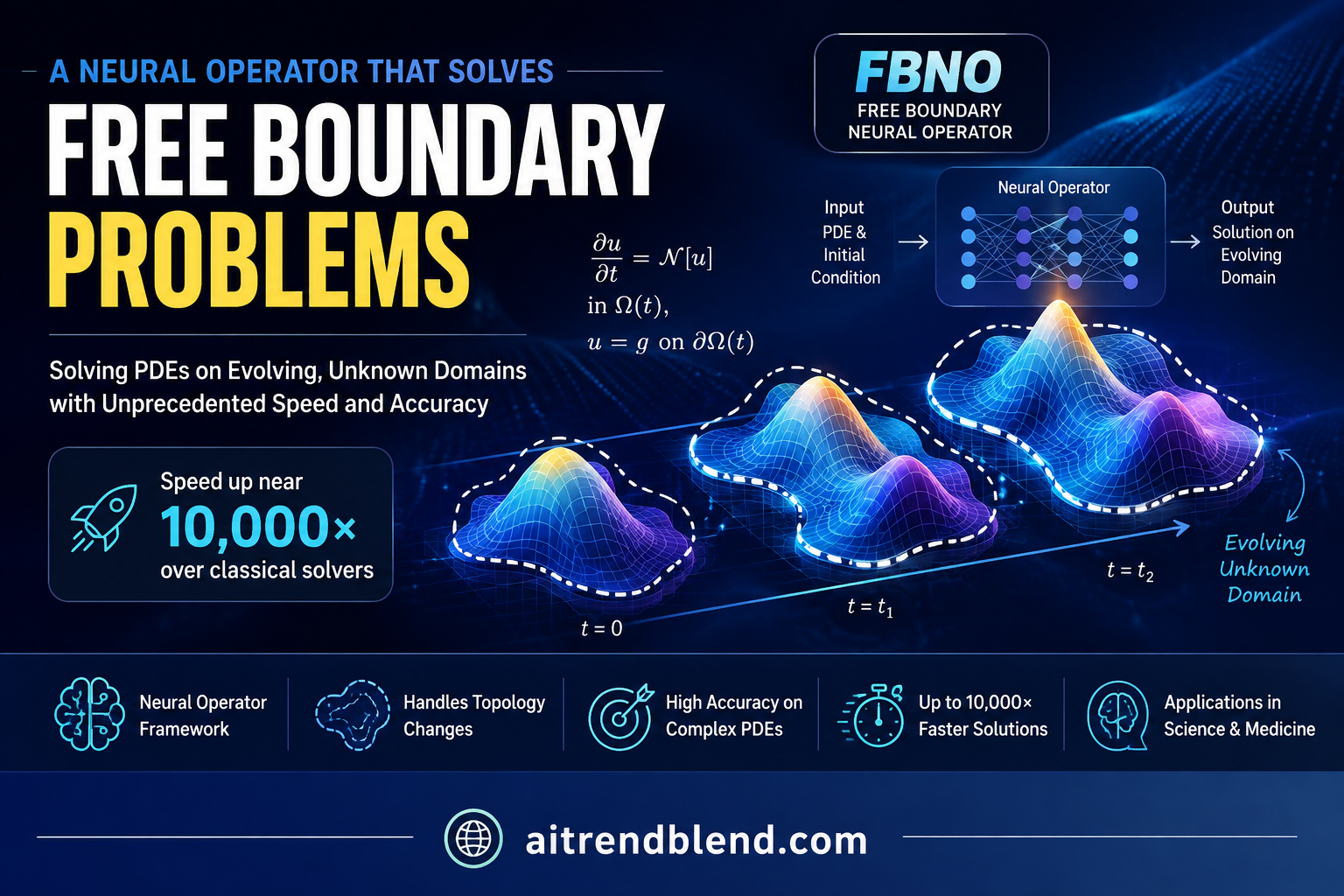
- The new method, FBNO, sidesteps the moving boundary by mapping the evolving shape onto a fixed reference shape through a learned diffeomorphism, then solving the easier problem on the fixed shape.
- The authors prove an approximation theorem, a mathematical guarantee that the method can in principle reach any target accuracy, which most deep learning solvers cannot claim.
- Across three very different tests, a classic phase change problem, a coupled multi physics system, and a tumour growth model, relative errors stayed within a few percent, and adding physics constraints cut testing error by more than ninety five percent.
- On the tumour case FBNO ran about ten thousand times faster than a traditional solver, turning a multi day simulation into a few seconds on a single graphics card.
What makes a free boundary problem so hard
Most of the equations that describe the physical world are solved on a fixed stage. You know the shape of the metal bar, the room, or the wing, and you compute how heat or air or stress plays out across it. A free boundary problem tears up that assumption. Here the stage itself is one of the unknowns. The equation governs what happens inside a region, but the edge of that region moves in response to what the equation is doing, and the two are locked together.
Melting ice is the textbook case, known as the Stefan problem. Heat flows into the ice, the ice turns to water, and the boundary between solid and liquid creeps forward. Where that boundary sits depends on the temperature, and the temperature depends on where the boundary sits. You cannot solve one without the other. The same tangle shows up all over science and engineering, in how a crack spreads through a solid, how sea ice grows in polar water, how plasma presses against the wall of a fusion reactor, and, most vividly, how a tumour expands into the tissue around it.
Traditional numerical methods handle these by tracking the moving boundary with a shifting mesh or by reformulating the whole thing on a fixed domain. Both work, and both are slow and delicate, which becomes a serious problem when you need to solve the same kind of equation hundreds of times over, once for each patient or each design. That repeated cost is what motivated the search for something faster.
Why the usual neural operators cannot help
Over the past decade a genuinely useful idea has taken hold in scientific computing. Rather than solve one equation at a time, train a neural operator to learn the whole mapping from inputs to solutions, so that once trained it can produce an answer for a new input almost instantly. The Fourier neural operator and DeepONet are the famous examples, and they have made some families of equations dramatically cheaper to solve. Our look at neural representations for scientific data covers a neighbouring idea in the same spirit of replacing brute force computation with a learned network.
There is a catch that stops all of them cold at the free boundary. A neural operator learns a mapping between function spaces defined over a given domain. The whole framework assumes the domain is fixed and known ahead of time. In a free boundary problem the domain is neither. It is unknown at the start and it changes as time passes. Feeding such a problem to a standard neural operator is like handing it a map with the coastline left blank and asking it to plot a route. The machinery has nowhere to stand.
The authors make this precise. The foundational approximation theorem that guarantees neural operators work at all requires the output functions to live on a fixed compact domain. A free boundary problem violates that requirement by its very nature, which means the existing theory does not even apply, let alone the methods built on it. Something new was needed.
The trick, borrowed from dynamical systems
The clever move is to stop fighting the moving boundary and instead map it away. FBNO, which stands for free boundary neural operator, leans on an old idea from the study of dynamical systems called topological conjugacy. Two systems are conjugate when one can be turned into the other by a continuous, reversible change of coordinates. If you can solve the easy one and you know the change of coordinates, you have solved the hard one for free.
FBNO treats the free boundary problem as a dynamical system whose state evolves over time, and it builds a second, tamer system that lives on a fixed reference domain that never changes shape. The reference shape is chosen to be a smooth deformation of the real evolving shape at every instant. Then two things get learned at once. A neural operator learns how the tame system flows forward on the fixed domain, and a second neural operator learns the deformation that bends the fixed shape into the real, moving one.
Read that equation from right to left and it tells a small story. Take the problem on the real moving shape, undo the deformation to land on the fixed reference shape, run the easy solver there, then reapply the deformation to get back. The deformation is the star, because it carries all the information about where the boundary actually is. Learn it well and the moving boundary stops being a wall and becomes just another thing the network predicts.
Keeping the deformation honest
For the trick to work, the deformation cannot fold the shape over on itself or tear it. In mathematical terms it must be a diffeomorphism, a smooth map that is smoothly reversible. The authors enforce this with a single clean constraint. The local stretching factor of the map, given by the determinant of its spatial derivative, must stay strictly positive everywhere.
This one inequality does a surprising amount of work. It preserves the inside and outside of the shape, it keeps the boundary directions sensible, and in the multi physics case it even doubles as a statement of mass conservation, because the same determinant equals the ratio of initial to current density. A physical law and a geometric safeguard turn out to be the same equation, which is the kind of coincidence that makes a method feel right.
FBNO does not predict the moving boundary directly. It learns a smooth, reversible deformation from a fixed reference shape to the real one, and that deformation quietly carries the boundary with it. Solving the equation then happens on the easy fixed shape.
A guarantee, not just a demonstration
Plenty of deep learning solvers work in practice and offer no promise that they will keep working as you ask for more accuracy. FBNO comes with a proof. The authors establish an approximation theorem for free boundary problems, a version of the universal approximation result tailored to this setting, showing that their construction can approximate the true solution operator to any accuracy you like.
The proof matters because it fills exactly the hole that blocked the standard theory. By routing everything through the diffeomorphism onto a fixed reference domain, the method restores the conditions the classical theorem needs, uniform continuity and boundedness over a compact domain, which the raw free boundary problem lacked. It is a rare case where a practical engineering fix and a clean theoretical fix are the same fix. Readers who enjoy the flavour of convergence guarantees for learning methods will find a kindred spirit in our piece on convergence theory for score based generative models, which chases the same kind of rigor in a different corner of the field.
Two ways to train it
FBNO can be taught in either of the two standard styles of scientific machine learning, and the choice depends on what you have.
When you have no solution data, you can train it in a self supervised, physics informed way. The network is pushed to obey the governing equations directly, through a composite loss that adds up several demands. Match the initial condition, respect the fixed boundaries, satisfy the free boundary condition, honour the underlying equation across the interior, and keep the deformation a valid diffeomorphism.
When you do have data, even a small amount, you can train it in a supervised way and let the diffeomorphism structure carry the rest. In the harder examples the authors combined both, learning from a modest set of low resolution simulations while the physics terms filled in what the data did not cover. That hybrid is where the method shines, because it stays accurate even when data is scarce, which is the usual situation in real problems.
Three tests, three kinds of hard
The proof is nice, but the paper earns attention by measuring FBNO on three problems that stress it in different ways.
| Problem | What makes it hard | How FBNO did |
|---|---|---|
| Stefan problem, phase change | A one dimensional interface that melts and moves | Temperature errors within about 1.5 percent, free boundary errors below 1 percent |
| Thermal structural coupling | Several physical fields interacting on a non convex shape | Mean relative errors near 0.1 percent for density and 1.3 percent for temperature, with physics constraints cutting test error by more than 95 percent |
| Tumour growth | A non convex, evolving three dimensional domain | Free boundary error near 0.37 percent and a speed up close to ten thousand times over a traditional solver |
The first test, the melting Stefan problem, is the honest baseline. It is the simplest free boundary problem and the one everyone checks first. FBNO reproduced both the temperature field and the moving interface with errors in the low single digit percents, and a nice detail emerged. The prediction error barely changed as the domain geometry varied, with deviations under a hundredth of a percent, which says the method genuinely learns the mapping rather than memorizing one shape.
The second test coupled heat, structure, and flow on awkward, non convex shapes. This is where the physics informed constraints proved their worth. Training with them cut testing error by more than ninety five percent compared with a purely data driven version, and the predictions stayed stable over time with no drift accumulating as the simulation ran forward. Getting several physical fields to agree on a moving domain is exactly the kind of thing that usually breaks a learned solver, and it held.
The work marks a turning point in free boundary simulations, as the use of neural networks unlocks both speed and precision. Long and colleagues, Nature Machine Intelligence, 2026
The tumour case, and where the excitement should stop
The third test is the one most likely to grab a headline, and it deserves both real interest and real caution. The authors modelled tumour growth, where a mass expands into surrounding tissue according to how nutrients diffuse and how cells divide and die. The growth term balances proliferation against death in a nonlinear way, and the tumour surface is a genuine free boundary that bulges into non convex shapes.
FBNO handled it. Across three different starting shapes it reconstructed the growing boundary with a relative error near four tenths of a percent, and it did so with a speed that is the real story here. The trained network produced a full growth trajectory in seconds on a single graphics card, where the equivalent traditional simulation needed more than two days on a sixteen node computing cluster. In throughput terms the neural operator handled about eighty five cases per second against a fraction of one case per second for the classical method. The authors frame this as a path toward real time, patient specific predictions of how a tumour and its nutrient supply might evolve.
Clinical translation gap
That framing is where careful reading has to take over from enthusiasm. A fast simulator of a mathematical tumour model is not a tool an oncologist can use on a patient, and the distance between the two is large. The model in this paper is a set of equations with tunable parameters, fed by synthetic and simulated data rather than by real scans of real people. Nothing in the study connects it to measured patient outcomes, to histology, or to the messy biology that governs how an actual cancer behaves.
The leap from a validated numerical method to a clinical decision aid would require a great deal more. It would need the model calibrated against real longitudinal imaging, tested prospectively on patients, checked for how its errors behave in the cases that matter most, and cleared through the regulatory process that any medical device faces. A method that runs ten thousand times faster is genuinely useful to the researchers who build and study these tumour models, and it may one day feed into clinical tools, but the paper demonstrates the engine, not the car. For a sense of what a more clinically grounded tumour growth model looks like, our analysis of a treatment aware diffusion model for glioma growth works directly from patient MRI, and even that stops well short of clinical deployment.
The tumour result is a speed and accuracy milestone for solving the underlying equations, not a clinical prediction about any real patient. The model was trained on simulated data, and turning it into anything a doctor could use would demand real patient validation and regulatory clearance.
Where the method falls short
The authors are candid about the limits, and a fair account has to include them.
The sharpest limitation is mathematical. FBNO assumes the moving boundary stays smooth. When a free boundary problem develops a singularity, such as a shock wave in a nonlinear system, the governing equations stop being well defined and the whole formulation breaks down. In those regimes, which include some of the most interesting physics, the method does not apply without being recast in a weaker mathematical form that sits outside this study.
There are practical limits too. The paper handles single phase problems, and extending it to two phase or multi phase systems, where two moving fronts interact, would require a separate learned map for each phase with careful coupling between them. The authors sketch this as future work rather than a solved problem. And while the approximation theorem guarantees that a good solution exists in principle, actually finding it through training runs into the usual troubles of scarce data and optimization getting stuck in poor local minima, so the theory promises more than any single training run can deliver.
Finally there is the cost that the impressive speed up hides. The ten thousand fold gain is measured after training. Getting there still requires generating training data and running a substantial optimization, which has to be counted in any honest tally of the total effort. The method pays for itself when you need to solve the same family of problems many times, and less so for a one off.
Why it still matters
Step back from the caveats and the contribution is clear. Free boundary problems were a blank spot on the map of what neural operators could touch, blocked not by a missing trick but by a theorem that did not fit. FBNO fills that spot with a method that is both provably sound and practically fast, and it does so in a way that does not care about the specific equation, which means it can be pointed at melting, at coupled multi physics, at tumour models, and at whatever comes next.
The deeper appeal is the marriage of an old mathematical idea with a modern learning method. Topological conjugacy has been a tool in dynamical systems for generations. Bolting it onto a neural operator turns a moving boundary from an obstacle into a learnable object, and it hands scientists a way to explore families of evolving domain problems at a speed that simply was not available before. That is the sort of quiet enabling advance that tends to matter more over time than any single flashy result.
A reference implementation
The code below is a compact, runnable sketch of the core idea. It builds a MIONet style operator with two branch networks and a shared trunk, uses it to predict a deformation from a fixed reference grid, computes the Jacobian determinant of that deformation with automatic differentiation, and trains against a toy target while penalizing any point where the determinant drops toward zero. The authors full code and data are linked under the block.
# Free boundary neural operator, compact reference sketch
# A MIONet style operator predicts a diffeomorphism chi over a fixed grid,
# and a Jacobian determinant penalty keeps that map invertible.

import torch
import torch.nn as nn

torch.manual_seed(0)


class MLP(nn.Module):
    def __init__(self, sizes):
        super().__init__()
        layers = []
        for i in range(len(sizes) - 1):
            layers.append(nn.Linear(sizes[i], sizes[i + 1]))
            if i < len(sizes) - 2:
                layers.append(nn.Tanh())
        self.net = nn.Sequential(*layers)

    def forward(self, x):
        return self.net(x)


class FBNO(nn.Module):
    # Two branches embed the inputs, the trunk embeds the reference coordinate,
    # and their Hadamard product summed over latent channels gives chi.
    def __init__(self, n_u0, n_psi, latent=64, out_dim=2):
        super().__init__()
        self.branch_u = MLP([n_u0, 128, latent * out_dim])
        self.branch_p = MLP([n_psi, 128, latent * out_dim])
        self.trunk = MLP([3, 128, latent * out_dim])   # input is (xi_x, xi_y, t)
        self.latent = latent
        self.out_dim = out_dim

    def forward(self, u0, psi, coord):
        b = coord.shape[0]
        bu = self.branch_u(u0).view(1, self.latent, self.out_dim)
        bp = self.branch_p(psi).view(1, self.latent, self.out_dim)
        tr = self.trunk(coord).view(b, self.latent, self.out_dim)
        # sum the triple product over the latent channels
        chi = (bu * bp * tr).sum(dim=1)                # shape [b, out_dim]
        return chi


def jacobian_det(chi, coord):
    # spatial Jacobian of chi with respect to (xi_x, xi_y), then its determinant
    dx = torch.autograd.grad(chi[:, 0].sum(), coord, create_graph=True)[0][:, :2]
    dy = torch.autograd.grad(chi[:, 1].sum(), coord, create_graph=True)[0][:, :2]
    det = dx[:, 0] * dy[:, 1] - dx[:, 1] * dy[:, 0]
    return det


def diffeo_penalty(det, delta=0.05):
    # push any determinant below the floor back up, otherwise no penalty
    return torch.relu(delta - det).mean()


if __name__ == "__main__":
    n_u0, n_psi = 16, 8
    model = FBNO(n_u0, n_psi)
    opt = torch.optim.Adam(model.parameters(), lr=1e-3)

    # one dummy sample, a grid of reference coordinates with a time stamp
    u0 = torch.randn(1, n_u0)
    psi = torch.randn(1, n_psi)
    gx, gy = torch.meshgrid(torch.linspace(0, 1, 12), torch.linspace(0, 1, 12), indexing="ij")
    t = torch.full_like(gx.reshape(-1, 1), 0.5)
    coord = torch.cat([gx.reshape(-1, 1), gy.reshape(-1, 1), t], dim=1)

    # toy target, a mild stretch of the identity to stand in for a real boundary
    target = coord[:, :2] * torch.tensor([1.3, 0.8]) + 0.05

    for step in range(400):
        coord_in = coord.clone().requires_grad_(True)
        chi = model(u0, psi, coord_in)
        det = jacobian_det(chi, coord_in)
        loss_fit = ((chi - target) ** 2).mean()
        loss = loss_fit + 10.0 * diffeo_penalty(det)
        opt.zero_grad()
        loss.backward()
        opt.step()
        if (step + 1) % 100 == 0:
            print(f"step {step + 1}  fit {loss_fit.item():.5f}  min_det {det.min().item():.3f}")
Go to the source
Read the peer reviewed paper and run the authors own code and data.
Read the paper Code on GitHubConclusion
The core achievement here is a neural operator that can finally handle free boundary problems, a class of equations that the whole neural operator toolkit had been unable to touch. By recasting the moving boundary as a learned deformation onto a fixed reference shape, FBNO turns an intractable setting into a tractable one, and it backs the construction with an approximation theorem that most learned solvers never bother to prove. Speed and a guarantee rarely travel together, and here they do.
The conceptual shift worth remembering is the reuse of topological conjugacy. Instead of predicting the boundary head on, the method learns a smooth, reversible map that carries the boundary along with it, and enforces that the map behaves through a single positive determinant constraint that also happens to encode a conservation law. It is an elegant piece of engineering, the kind where the mathematical safeguard and the physical law turn out to be the same line.
The approach travels well because it is deliberately agnostic to the equation and the neural architecture. The same framework solved a melting interface, a coupled multi physics system, and a growing tumour, and it slotted into a DeepONet style backbone without special pleading. That generality is arguably the larger contribution, since it opens a whole category of evolving domain problems to fast learned solvers rather than solving one narrow instance.
The honest limits keep the celebration measured. The method assumes a smooth boundary and breaks where singularities form, it handles a single phase rather than the harder multi phase case, and its headline speed up is a post training figure that a full accounting must weigh against the cost of data and optimization. The tumour result in particular is a milestone in solving the underlying equations, not a clinical prediction about any real person, and the road from a fast simulator to a tool a doctor could trust runs through patient data and regulation that this work does not attempt.
Future directions follow naturally. Extend the method to multi phase fronts, find a formulation that survives singularities, and, in the biomedical direction, connect these fast models to real imaging so that the speed can eventually serve the clinic rather than only the equation. If those steps hold up, a problem that took a century to compute quickly becomes something a laptop can explore, and that shift tends to change what questions people are willing to ask.
Frequently asked questions
What is a free boundary problem?
It is a type of equation where the region it is solved on is unknown and changes over time, and the motion of that region is coupled to the solution itself. Melting ice, spreading cracks, and growing tumours are all examples.
Why can standard neural operators not solve these problems?
Neural operators such as the Fourier neural operator and DeepONet assume the domain is fixed and known in advance. A free boundary problem has a domain that is neither, so the frameworks and even the theory behind them do not apply.
How does FBNO get around the moving boundary?
It maps the evolving shape onto a fixed reference shape through a learned smooth and reversible deformation, solves the easier problem on the fixed shape, then maps back. The deformation carries the boundary, so the network never has to predict it directly.
Is the tumour growth result a medical tool?
No. It is a fast and accurate way to solve a mathematical tumour growth model on simulated data. It is not validated on real patients and is not a diagnostic or treatment tool, so it should not be read as clinical advice.
How much faster is it than traditional methods?
On the tumour growth case the trained network was about ten thousand times faster than a traditional solver, producing a full growth trajectory in seconds on a single graphics card where a computing cluster needed more than two days.
Can the code and data be reproduced?
Yes. The authors released their code and data on GitHub, Zenodo, and Code Ocean under an open licence, so the Stefan, thermal structural, and tumour growth results can be reproduced and extended.