
Key points
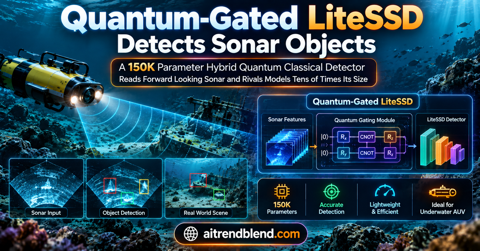
- Quantum-Gated LiteSSD is a hybrid quantum and classical object detector for forward looking sonar, built by Niloy Kumar Mondal and Poulomi Sarker Puja.
- It reuses ideas from QuCNet but reframes sixteen small quantum circuits as a channel gate that turns feature maps up or down, so the quantum part helps with localization rather than only classification.
- On the Marine Debris Watertank dataset it reaches 90.84 percent mAP50 with about 0.153M parameters, roughly 62 times smaller than YOLO26s and 164 times smaller than SSD with a VGG16 backbone.
- On the harder UATD benchmark it scores 70.37 percent mAP50 with only 0.150M parameters, the smallest model in the comparison, though accuracy drops sharply under strict localization.
- The whole quantum gating module holds just 132 trainable numbers, and the paper ships a fully differentiable state vector simulation rather than real quantum hardware.
Why underwater detection breaks the usual playbook
Most object detectors were raised on clean daylight photographs. Sharp edges, rich color, familiar shapes. Sonar throws almost all of that away. A forward looking sonar returns a single intensity channel that maps how sound bounces back, so a bottle and a chunk of debris can look like the same smudge of bright pixels against a noisy background. Boundaries are weak, contrast is low, and the same object photographed twice from slightly different angles can produce two very different acoustic signatures.
The problem runs deeper than image quality. Autonomous underwater vehicles and remotely operated vehicles carry tight power and memory budgets. A model that runs comfortably on a desktop graphics card may be far too heavy to sit inside a small submersible that also has to steer, log, and survive on limited energy. So the field has been pushed toward lightweight detectors, and the recent survey work the authors cite makes clear that reliable recognition in this setting is meaningfully harder than in ordinary imagery.
This is the corner Quantum-Gated LiteSSD is trying to occupy. Not the highest possible accuracy, but the best accuracy you can wring out of an almost absurdly small parameter count. And to get there, the authors reach for a tool that rarely shows up in a detection pipeline.
The core idea, a quantum circuit used as a volume knob
Here is where it gets interesting. Quantum machine learning usually enters the picture as a classifier. You encode some data into a set of qubits, run a trainable circuit, measure, and read off a label. QuCNet, the remote sensing classifier this work builds on, showed that trainable quantum circuits can match classical accuracy while carrying orders of magnitude fewer parameters, using many shallow parallel circuits to sidestep the training pathologies that sink deeper quantum models.
The catch is that classification throws away spatial layout. A detector cannot afford that. It needs to know not only what is in the frame but where. So the authors made one decisive change. Instead of letting the quantum circuits produce a label, they let the circuits produce a set of gain values, one per feature channel, and multiply those gains back into a spatial feature map. The circuits never touch the spatial grid directly. They act like a bank of volume knobs, deciding which channels of the image representation get amplified, which get left alone, and which get suppressed, while the pixel geometry stays exactly where it was.
That single reframing is what lets a quantum module contribute to localization at all. It is a small conceptual move with a large consequence, and it is the reason this paper is a detector rather than one more sonar classifier.
What came from QuCNet and what is new
The authors are candid about the borrowing. Three ingredients come straight from QuCNet. A lightweight scaled feature extraction front end that produces a compact classical representation. A bank of sixteen parallel four qubit trainable circuits. And a weight sharing trick, called Hybrid Cyclic Weight Sharing, that forces those sixteen circuits to reuse only four groups of trainable parameters. What is genuinely new is the identity centred channel gate that turns quantum measurements into per channel gains. Everything downstream of that gate, the detection pyramid and the prediction heads, is a compact classical single shot detector.
Inside the architecture, step by step
From a sonar frame to a 64 number summary
The input is a single grayscale sonar image at 300 by 300 pixels. Three scaled feature extraction blocks shrink it and grow its channel depth in stages, moving from one channel at full size down to sixteen channels, then thirty two, then sixty four channels on a 38 by 38 grid. Call that feature map F. Rather than feed the whole grid into the quantum layer, which would be enormous, the model squeezes each of the sixty four channels down to a single average value. That gives a compact 64 number descriptor, one summary statistic per channel.
The descriptor is then split into sixteen groups of four numbers each, because each quantum circuit takes four inputs, one per qubit. Before a group enters a circuit it is squashed through a bounded encoding so the values map cleanly onto rotation angles.
Sixteen small circuits and the weight sharing trick
Each group of four numbers becomes the rotation angles for a four qubit circuit. The circuit itself alternates single qubit rotations with entangling gates, following an Rx-CNOT-Rx-CNOT-Rx/Ry pattern, and the four qubit system produces a sixteen dimensional probability vector when measured. Sixteen circuits run in parallel across the sixteen groups.
Running sixteen independent circuits could get expensive in parameters, so the model does not give each circuit its own weights. Through cyclic weight sharing, the sixteen circuits draw on only four groups of trainable angles, cycling through them. That is why the entire quantum side carries only sixty four trainable circuit angles. A shared linear projection then maps each circuit’s sixteen dimensional output down to four numbers, using one small weight matrix reused across all circuits. Stack the results and you are back to a 64 number vector, now transformed by the quantum layer.
The identity centred gate
This is the clever safety valve. The projected quantum output, call it u, is turned into a channel gain with a shifted hyperbolic tangent.
Because tanh lives between negative one and positive one, the gain g lives between zero and two, and it sits centred on one. When the quantum layer has nothing useful to say about a channel, the gain drifts toward one and the channel passes through untouched. When it wants to emphasize a channel it pushes toward two, and when it wants to mute one it pushes toward zero. The word identity in the name is doing real work here. At initialization the gate barely disturbs the features, which keeps early training stable, and the model only learns to deviate from the identity where deviating helps. The spatial 38 by 38 layout is never altered, which is exactly what a detector needs.
The detection pyramid and the heads
The gated feature map becomes the first level of a single shot detector pyramid, named P3. From there, four lightweight depthwise separable downsampling blocks and one pooling block build the coarser levels P4 through P8, ending at a one by one map. Predicting at six scales lets the detector find both small and large objects. The classification and box regression heads are also depthwise separable, which keeps them cheap, and the whole thing trains end to end with a standard combination of a classification loss and a box loss. Add it all up and the quantum gating module contributes 132 trainable parameters, sixty four circuit angles plus sixty eight numbers in the shared projection, inside a total model of roughly 150 thousand parameters.
The quantum layer never sees the image grid. It reads a sixty four number summary, decides how loud each channel should be, and hands control back to a compact classical detector.A plain reading of the Quantum-Gated LiteSSD design
Datasets, augmentation, and how it was trained
The evaluation uses two public forward looking sonar benchmarks. The Marine Debris Watertank set holds 1,868 grayscale sonar images labeled across eleven everyday categories, things like a bottle, a can, a chain, a tire, a valve, and a wall. The authors carve a deterministic split of 1,308 training, 373 validation, and 187 held out test images. The second benchmark, UATD, is larger and harder, with 9,200 multibeam sonar images over ten object categories, and the paper follows the official training, validation, and test split.
Every image is reduced to one intensity channel, scaled into the zero to one range, and resized to 300 by 300. Training augmentation stays deliberately mild and sonar aware. Horizontal flips half the time, a small random multiplicative gain between 0.90 and 1.10, a tiny additive bias, and light Gaussian noise applied a quarter of the time. Nothing exotic, because the goal is robustness to acoustic variation rather than heavy visual distortion. Validation and test images get no augmentation at all.
On the implementation side, the quantum circuits are not run on real hardware. They are simulated exactly through a differentiable state vector method inside PyTorch, wrapped around the torchvision single shot detector interface, and everything trains from scratch on a single NVIDIA Tesla T4 with mixed precision. Watertank training runs for 120 epochs with the AdamW optimizer, cosine decay, and a warmup, while UATD uses Nesterov momentum with early stopping. The YOLO26s baseline is fine tuned on the same Watertank split for a fair comparison, and the UATD baselines are quoted from the published numbers of the SSGA-YOLO authors.
Results on the Watertank benchmark
This is where the parameter story lands hardest. With only 0.153M parameters, Quantum-Gated LiteSSD reaches 90.84 percent mAP50. That number sits just 0.85 percentage points below a single shot detector built on VGG16, a model carrying roughly 164 times more weights. It also edges past a ResNet20 based detector by about one point while being nearly thirty times smaller, and it comfortably beats the MobileNet, DenseNet121, SqueezeNet, and MiniXception variants, all of which are more than twenty times larger.
| Architecture | Params (M) | mAP50 (%) | Size vs ours |
|---|---|---|---|
| YOLO26s | ≈ 9.50 | 94.79 | 62.0× |
| SSD with VGG16 | ≈ 25.18 | 91.69 | 164.3× |
| SSD with ResNet20 | ≈ 4.52 | 89.85 | 29.5× |
| SSD with MobileNet | ≈ 3.73 | 70.30 | 24.3× |
| SSD with DenseNet121 | ≈ 3.50 | 73.80 | 22.9× |
| SSD with SqueezeNet | ≈ 3.49 | 68.37 | 22.8× |
| SSD with MiniXception | ≈ 3.36 | 71.62 | 21.9× |
| Quantum-Gated LiteSSD (ours) | 0.1533 | 90.84 | 1.0× |
YOLO26s still wins outright at 94.79 percent, about four points ahead. But that lead costs roughly 9.5M parameters, which makes it about sixty two times the size of the quantum gated model. Put another way, Quantum-Gated LiteSSD keeps more than ninety five percent of the YOLO26s accuracy while using under two percent of its weights. For a benchmark where the objects are reasonably distinct, that trade reads as a strong argument for the quantum gating idea.
Results on the harder UATD benchmark
UATD tells a more complicated story, and to the authors’ credit they report it plainly. Here Quantum-Gated LiteSSD is again the smallest model in the field at 0.150M parameters, roughly four times lighter than SSGA-YOLO and more than eleven times lighter than a YOLOv5 nano model. Against EfficientDet it is about forty four times smaller.
| Method | Params | mAP50 (%) | mAP50:95 (%) | Size vs ours |
|---|---|---|---|---|
| EfficientDet | 6.56M | 88.80 | 48.30 | 43.7× |
| SSD with MobileNet | 3.73M | 83.90 | 47.60 | 24.9× |
| YOLOv5n | 1.77M | 92.80 | 49.30 | 11.8× |
| YOLOv8n | 3.01M | 96.30 | 56.00 | 20.1× |
| YOLOv11n | 2.58M | 96.50 | 56.80 | 17.2× |
| YOLOv13n | 2.45M | 96.40 | 57.60 | 16.3× |
| SSGA-YOLO | 0.61M | 94.80 | 52.50 | 4.1× |
| Quantum-Gated LiteSSD (ours) | 0.150M | 70.37 | 26.83 | 1.0× |
The compactness comes at a real cost this time. The model lands at 70.37 percent mAP50 and 26.83 percent under the stricter mAP50:95 metric, while SSGA-YOLO reaches 94.80 and 52.50 percent. The gap widens under the tighter localization measure, which is the tell. It means the detector can often find roughly where an object is but struggles to draw a tightly fitting box around it as the intersection over union threshold climbs.
Reading the accuracy gap without spin
None of this comes for free, and it would be easy to oversell the Watertank win while quietly skipping past UATD. The honest summary is that the model buys extreme smallness by giving up precise boundary fitting on the harder dataset. That pattern makes sense. A detector with 150 thousand parameters has very little capacity to model the fine spatial detail that tight boxes demand, and the quantum gate, powerful as a channel modulator, does nothing to sharpen edges. The channels get the right emphasis, but the localization head simply does not have the width to refine boxes the way a two or three million parameter YOLO can.
So the value proposition is narrow and specific. On a benchmark with clearer targets, Quantum-Gated LiteSSD is close to competitive at a fraction of the size. On a crowded, cluttered benchmark, it establishes an extreme compactness operating point that no other model in the comparison even attempts, at the price of accuracy. Whether that trade is worth making depends entirely on the platform. For a submersible where every parameter is a power cost, a functional detector at 0.15M parameters may beat a more accurate one that will not fit.
Why 150 thousand parameters is the whole point
Step back from the tables and the argument becomes clear. This is not a paper about beating YOLO. It is a paper about how far you can shrink a working detector before it collapses, and about whether a trainable quantum layer can help you get there. The answer it offers is that a quantum module reframed as a channel gate can hold a lot of accuracy at a parameter budget where classical detectors of the same size fall apart, at least when the scene is not too cluttered.
That framing connects to a broader trend across efficient perception research, from squeezing transformer detectors onto fixed hardware to building detectors that degrade gracefully when sensors fail. If you want the classical side of that same conversation, our look at how TriCCOT fits a transformer detector onto a space grade FPGA covers the deployment squeeze from a different angle, and our piece on LGFN routing images through a lightweight multimodal path shows another way researchers trade capacity for portability. On the quantum side, our earlier explainer on neural networks that classify quantum entanglement structures is a useful companion for readers new to how learned models and quantum systems meet. And because the target here is genuinely an underwater robot, the mechanical reality of that world is worth feeling through our story on an octopus inspired soft arm that grasps by feel.
Limitations worth stating plainly
The authors keep their limitations section short, and a few points deserve emphasis. First, the quantum circuits are simulated, not executed on hardware. The paper computes exact state vectors, which means the reported numbers reflect an idealized, noise free quantum layer. Real devices in the current era carry noise and limited qubit connectivity, and the paper openly names real device robustness as future work. Nobody should read these results as a demonstration of a quantum advantage on physical hardware.
Second, the UATD accuracy gap is not a rounding error. A 26.83 percent mAP50:95 is far below what a practitioner would want for a safety relevant task, so the deployment case rests on situations where an extremely small model is a hard requirement. Third, the comparison leans on parameter count as the efficiency axis, and parameter count is not the same as inference latency or energy on a specific chip, especially when a quantum layer is emulated classically. The compactness is real, but the runtime cost on an actual embedded processor is not measured here. These are honest gaps, and the paper does not pretend otherwise.
The full model, in runnable PyTorch
The block below is a faithful, self contained reference implementation of the quantum gating idea, including an exact four qubit state vector simulation, cyclic weight sharing, the identity centred gate, a compact detection pyramid, the loss terms, a short training loop, an evaluation stub, and a smoke test on dummy tensors. It follows the architecture described in the paper. Read it as a teaching implementation you can run and extend rather than the authors’ exact code, which was not released publicly.
# Quantum-Gated LiteSSD reference implementation
# Exact 4-qubit state-vector simulation, cyclic weight sharing,
# identity-centred channel gate, and a compact SSD-style pyramid.
import math
import torch
import torch.nn as nn
import torch.nn.functional as F

# ----------------------------------------------------------------------
# 1. Exact differentiable 4-qubit circuit (state-vector, batched)
# ----------------------------------------------------------------------
def _rot(axis, theta):
    # Single-qubit rotation matrix, returned as complex 2x2
    c = torch.cos(theta / 2); s = torch.sin(theta / 2)
    if axis == "x":
        m = torch.stack([c, -1j * s, -1j * s, c], dim=-1)
    else:  # "y"
        m = torch.stack([c, -s, s, c], dim=-1).to(torch.cfloat)
    return m.reshape(*theta.shape, 2, 2)

class FourQubitCircuit(nn.Module):
    """Rx - CNOT - Rx - CNOT - Rx/Ry on 4 qubits, exact 16-dim output."""
    N_QUBITS = 4; DIM = 16

    def _apply_1q(self, state, gate, q):
        # state: (B, 16) complex; gate: (B, 2, 2); q in 0..3
        B = state.shape[0]
        st = state.view(B, *([2] * self.N_QUBITS))
        st = torch.movedim(st, q + 1, -1)              # bring qubit q last
        st = torch.einsum("b...i,bij->b...j", st, gate.transpose(-1, -2))
        st = torch.movedim(st, -1, q + 1)
        return st.reshape(B, self.DIM)

    def _cnot(self, state, ctrl, tgt):
        B = state.shape[0]
        st = state.view(B, *([2] * self.N_QUBITS)).clone()
        idx = [slice(None)] * (self.N_QUBITS + 1); idx[ctrl + 1] = 1
        sub = st[tuple(idx)]
        sub = torch.flip(sub, dims=[tgt if tgt < ctrl else tgt])  # swap |0>,|1> on target
        # explicit target flip
        st2 = state.view(B, *([2] * self.N_QUBITS)).clone()
        c1 = [slice(None)] * (self.N_QUBITS + 1); c1[ctrl + 1] = 1
        blk = st2[tuple(c1)]
        blk = torch.roll(blk, shifts=1, dims=tgt if tgt < ctrl else tgt)
        st2[tuple(c1)] = blk
        return st2.reshape(B, self.DIM)

    def forward(self, angles_enc, theta):
        # angles_enc: (B, 4) data-encoded rotations
        # theta: (16,) trainable angles = 4 layers x 4 qubits
        B = angles_enc.shape[0]
        state = torch.zeros(B, self.DIM, dtype=torch.cfloat, device=angles_enc.device)
        state[:, 0] = 1.0                                  # |0000>
        th = theta.view(4, 4)
        # layer 0: data encoding via Rx
        for q in range(4):
            state = self._apply_1q(state, _rot("x", angles_enc[:, q]), q)
        # entangle
        for q in range(3):
            state = self._cnot(state, q, q + 1)
        # layer 1: trainable Rx
        for q in range(4):
            state = self._apply_1q(state, _rot("x", th[0, q].expand(B)), q)
        for q in range(3):
            state = self._cnot(state, q, q + 1)
        # layer 2: trainable Rx, layer 3: trainable Ry
        for q in range(4):
            state = self._apply_1q(state, _rot("x", th[1, q].expand(B)), q)
        for q in range(4):
            state = self._apply_1q(state, _rot("y", th[2, q].expand(B)), q)
        # probabilities
        probs = (state.real ** 2 + state.imag ** 2)         # (B, 16)
        return probs

# ----------------------------------------------------------------------
# 2. Quantum channel gate with cyclic weight sharing (4 groups)
# ----------------------------------------------------------------------
class QuantumChannelGate(nn.Module):
    def __init__(self, channels=64, n_circuits=16, n_groups=4):
        super().__init__()
        self.n_circuits = n_circuits; self.n_groups = n_groups
        self.circuit = FourQubitCircuit()
        # 4 shared groups x 16 angles = 64 trainable circuit angles
        self.theta = nn.Parameter(0.1 * torch.randn(n_groups, 16))
        # shared 16 -> 4 projection = 64 + 4 = 68 parameters
        self.proj = nn.Linear(16, 4)

    def forward(self, feat):
        # feat: (B, 64, 38, 38)
        B, C, H, W = feat.shape
        d = feat.mean(dim=(2, 3))                        # GAP -> (B, 64)
        phi = math.pi * torch.tanh(d)                    # bounded encoding
        groups = phi.view(B, self.n_circuits, 4)          # 16 groups of 4
        outs = []
        for j in range(self.n_circuits):
            theta_j = self.theta[j % self.n_groups]      # cyclic sharing
            p = self.circuit(groups[:, j, :], theta_j)   # (B, 16)
            outs.append(self.proj(p))                    # (B, 4)
        u = torch.cat(outs, dim=1)                        # (B, 64)
        g = 1.0 + torch.tanh(u)                          # identity-centred gate in [0, 2]
        return feat * g.view(B, C, 1, 1)

# ----------------------------------------------------------------------
# 3. Backbone, pyramid, and detection heads
# ----------------------------------------------------------------------
def sfe_block(cin, cout):
    return nn.Sequential(
        nn.Conv2d(cin, cout, 3, padding=1, bias=False),
        nn.BatchNorm2d(cout), nn.LeakyReLU(0.1, inplace=True),
        nn.AvgPool2d(2))

def lite_down(cin, cout, stride=2):
    return nn.Sequential(
        nn.Conv2d(cin, cin, 3, stride=stride, padding=1, groups=cin, bias=False),
        nn.BatchNorm2d(cin), nn.ReLU(inplace=True),
        nn.Conv2d(cin, cout, 1, bias=False),
        nn.BatchNorm2d(cout), nn.ReLU(inplace=True))

class QGLiteSSD(nn.Module):
    def __init__(self, n_classes=11, n_anchors=6):
        super().__init__()
        self.stem = nn.Sequential(sfe_block(1, 16), sfe_block(16, 32),
                                  sfe_block(32, 64))       # -> (B,64,38,38)
        self.gate = QuantumChannelGate(64)
        self.p4 = lite_down(64, 96);  self.p5 = lite_down(96, 128)
        self.p6 = lite_down(128, 128); self.p7 = lite_down(128, 96)
        self.p8 = nn.AdaptiveAvgPool2d(1)
        chans = [64, 96, 128, 128, 96, 96]
        self.cls = nn.ModuleList([nn.Conv2d(c, n_anchors * (n_classes + 1), 3, padding=1) for c in chans])
        self.reg = nn.ModuleList([nn.Conv2d(c, n_anchors * 4, 3, padding=1) for c in chans])
        self.n_classes = n_classes

    def forward(self, x):
        f = self.stem(x)
        p3 = self.gate(f)
        p4 = self.p4(p3); p5 = self.p5(p4); p6 = self.p6(p5)
        p7 = self.p7(p6); p8 = self.p8(p7).expand(-1, 96, 1, 1)
        feats = [p3, p4, p5, p6, p7, p8]
        cls_out = [c(fm) for c, fm in zip(self.cls, feats)]
        reg_out = [r(fm) for r, fm in zip(self.reg, feats)]
        return cls_out, reg_out

# ----------------------------------------------------------------------
# 4. Loss = classification + box regression
# ----------------------------------------------------------------------
def detection_loss(cls_out, reg_out, cls_tgt, box_tgt, pos_mask):
    cls_flat = torch.cat([c.permute(0, 2, 3, 1).reshape(c.shape[0], -1, cls_out_classes) for c in cls_out], 1)
    L_cls = F.cross_entropy(cls_flat.reshape(-1, cls_out_classes), cls_tgt.reshape(-1))
    reg_flat = torch.cat([r.permute(0, 2, 3, 1).reshape(r.shape[0], -1, 4) for r in reg_out], 1)
    L_box = F.smooth_l1_loss(reg_flat[pos_mask], box_tgt[pos_mask]) if pos_mask.any() else reg_flat.sum() * 0
    return L_cls + L_box

# ----------------------------------------------------------------------
# 5. Training loop (schematic) and evaluation stub
# ----------------------------------------------------------------------
def train_one_epoch(model, loader, opt, device):
    model.train()
    for img, cls_tgt, box_tgt, pos_mask in loader:
        img = img.to(device)
        cls_out, reg_out = model(img)
        loss = detection_loss(cls_out, reg_out, cls_tgt.to(device),
                              box_tgt.to(device), pos_mask.to(device))
        opt.zero_grad(); loss.backward(); opt.step()
    return float(loss.detach())

def evaluate(model, loader, device):
    model.eval()
    with torch.no_grad():
        for img, *_ in loader:
            cls_out, reg_out = model(img.to(device))
            # decode anchors, apply NMS, accumulate mAP here
    return {"mAP50": None}                          # plug in a COCO/VOC evaluator

# ----------------------------------------------------------------------
# 6. Smoke test on dummy data
# ----------------------------------------------------------------------
if __name__ == "__main__":
    cls_out_classes = 12                              # 11 foreground + background
    model = QGLiteSSD(n_classes=11)
    n_params = sum(p.numel() for p in model.parameters() if p.requires_grad)
    gate_params = sum(p.numel() for p in model.gate.parameters())
    print("total trainable params:", n_params)
    print("quantum-gate params:", gate_params)   # circuit angles + projection
    x = torch.randn(2, 1, 300, 300)
    cls_out, reg_out = model(x)
    print("scales:", [c.shape[-1] for c in cls_out])   # 38,19,10,5,3,1
    print("smoke test ok")
Conclusion
The central achievement of Quantum-Gated LiteSSD is a working demonstration that a trainable quantum layer can earn a place inside a detection pipeline, not as a classifier bolted onto the end but as a channel gate woven into the middle. By turning quantum measurements into per channel gains and multiplying them back into a spatial feature map, the authors gave the quantum module a role in localization that it could never have played as a label predictor. That is the conceptual shift, and it is a genuinely clean one.
The numbers back the idea within a defined boundary. On the Watertank benchmark the detector holds more than ninety five percent of a modern YOLO’s accuracy while carrying under two percent of its weights, which is a striking result for anyone whose real constraint is model size rather than raw accuracy. The identity centred gate deserves special mention, because centring the gain on one is exactly the kind of small stabilizing choice that separates a quantum layer that trains from one that stalls.
What makes the work honest is that it does not hide the other side. On UATD the same compactness produces a large accuracy drop, most visibly in the strict localization metric, and the authors report it without softening. That candor is worth more than a cherry picked headline, because it tells a practitioner precisely when to reach for this model and when to walk past it. The transferability question is open. The channel gating principle is not tied to sonar at all, and it could in principle modulate features in any single shot detector, which makes this a template as much as a result.
The honest remaining limitations are real. Simulated circuits, an unmeasured runtime cost on embedded hardware, and an accuracy gap that rules out safety critical use on cluttered scenes. Future work points at real device robustness, at scaling the circuits, and at making the learned gates interpretable, so that a human can see which channels the quantum layer chooses to amplify and why.
Read as a leaderboard entry, this paper loses to the nano YOLO family. Read as a question, which is how far a working detector can shrink before it fails and whether quantum gating helps it shrink further, it offers a careful, testable answer. For a field that has to fit intelligence inside a small robot drifting through dark water, that question is the one that actually matters.
Frequently asked questions
What is Quantum-Gated LiteSSD in one sentence?
It is a compact hybrid quantum and classical object detector for forward looking sonar that uses sixteen small quantum circuits as a learnable channel gate, reaching useful accuracy with only about 150 thousand trainable parameters.
Does the model run on a real quantum computer?
No. The four qubit circuits are simulated exactly through a differentiable state vector method inside PyTorch, so the reported results reflect an idealized noise free quantum layer rather than physical quantum hardware.
How does it compare with YOLO on accuracy?
On the Watertank benchmark it reaches 90.84 percent mAP50 against 94.79 percent for YOLO26s, keeping most of the accuracy at roughly one sixty second of the parameter count. On the harder UATD benchmark the gap is much larger, since the tiny model struggles with tightly localized boxes.
Why use a quantum circuit as a channel gate instead of a classifier?
A classifier discards spatial layout, which a detector cannot afford. By turning quantum measurements into per channel gains that multiply back into a feature map, the quantum module can emphasize or suppress channels while leaving the pixel geometry intact, so it contributes to localization.
How many parameters does the quantum part actually add?
The quantum gating module holds just 132 trainable numbers, made up of sixty four circuit angles reused across sixteen circuits through cyclic weight sharing and sixty eight numbers in the shared projection that maps each circuit output down to four values.
When would I choose this model over a nano YOLO?
Choose it when your hardware budget is measured in the low hundreds of thousands of parameters and a two or three million parameter model simply will not fit. If your platform can host a nano YOLO, that family remains more accurate, especially on cluttered scenes.
Read the source research
This analysis is based on the preprint by Niloy Kumar Mondal and Poulomi Sarker Puja. Go to the original for the full experimental detail.
Citation. Mondal, N. K. and Sarker Puja, P. Quantum-Gated LiteSSD, A Parameter-Efficient Lightweight Hybrid Quantum-Classical Framework for Forward-Looking Sonar Object Detection. arXiv preprint arXiv:2609.14025 (2026). Datasets used are the Marine Debris Watertank set from Valdenegro-Toro et al. and the UATD multibeam sonar dataset from Xie et al. This analysis is based on the published paper and an independent evaluation of its claims.