
- Deep snake
- Mamba2 SSD
- Contour segmentation
- Vision language
- Spine MRI and CT
- Abdominal CT
- PyTorch
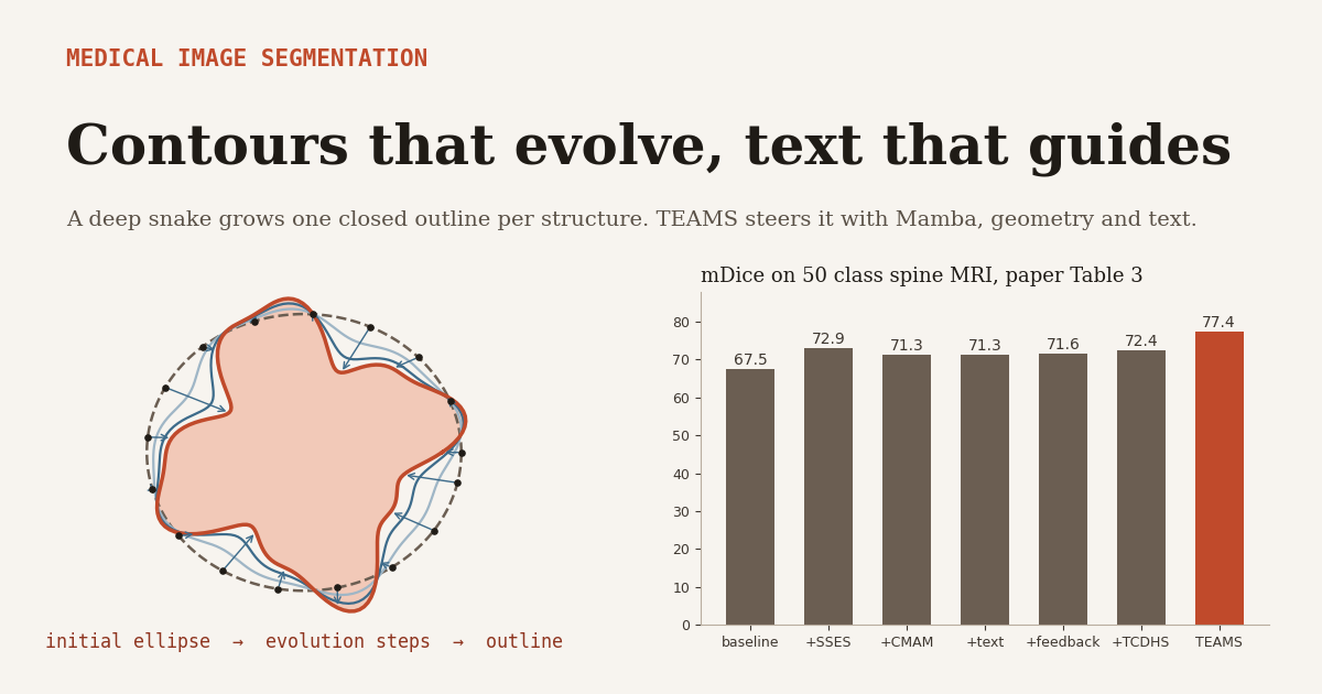
A radiologist opens a whole spine MRI of a patient with suspected metastatic disease. There are twenty five vertebral bodies and two dozen discs to outline, from the sacrum up to the first cervical vertebra, plus the spinal cord. A pixel classifier will usually get most of them right. It will also, now and then, punch a hole in the middle of a vertebral body, merge two discs into one blob, or label the T8 vertebra as T7 because the two look almost identical. Every one of those errors has to be found and fixed by hand.
A team led by Shen Zhao at Sun Yat-sen University, with collaborators at Zhejiang University and Case Western Reserve University, took a different route. Their model, TEAMS, does not colour pixels at all. It detects each structure, drops a closed contour around it, and lets that contour crawl toward the boundary, guided by a Mamba state space model, a sentence of anatomical text and a feedback loop from the finished contours back to the detector. This piece works through how each of those parts is built, what the published numbers support, and where the mathematics raises questions the paper does not answer.
Key points
- TEAMS is a deep snake model. It segments each organ as an ordered ring of points that evolves from a detection box to the boundary, which rules out holes and jagged fragments by construction.
- Its evolution step runs a Mamba2 style state space model along the contour in both directions and across previous evolution steps, with an exponential decay of 0.5 per step over history.
- A contour morphology prior nudges the Mamba attention mask toward points with high curvature and sharp corners. Our analysis shows that prior can never exceed about 0.27 and mostly pushes the model toward short range mixing.
- Task level and organ level text prompts from a frozen ClinicalBERT encoder, plus a stop gradient consistency loss from a second detector, reduce missed detections.
- On five datasets TEAMS led on four, including a relative mDice gain of 6.9 percent over the next best method on a private 50 class spine MRI set. It ranked second on PanNuke nuclei.
- All results are slice level research benchmarks. The paper reports no prospective or clinical validation, and one of the five datasets cannot be shared.
This article explains a published computer science paper about automatic image segmentation. It is not medical advice, not a diagnosis and not a treatment recommendation, and the model described is a research prototype, not an approved medical device. Anyone with questions about their own scans or health should speak with a qualified clinician.
Why Pixels Make Illogical Mistakes
Most medical segmentation networks, from the original U-Net through TransUNet and nnU-Net, answer one question for every pixel. Which class does this pixel belong to? That framing is powerful, and it is also blind to objects. Nothing in a per pixel loss says that a vertebral body is one connected piece with a smooth outline, so the network can produce holes, disconnected islands and ragged edges whenever local appearance is ambiguous. The authors call these illogical errors, and anyone who has corrected automatic contours in a planning system will recognise them.
Snake models attack the problem from the other side. The classical active contour of Michael Kass, Andrew Witkin and Demetri Terzopoulos in 1988 represented a boundary as a curve that moves to minimise an energy built from image gradients and smoothness. In 2020, Sida Peng and colleagues made the idea fully learnable with Deep Snake. A detector proposes a box, an initial contour is placed inside it, and a network repeatedly predicts an offset for every contour point. The output is always a single closed polygon per object, which is the property radiologists care about.
Deep snakes have their own weaknesses. The paper lists three. Contours can fail to evolve correctly when shapes vary a lot. They tend to smooth away fine detail such as the pointed edge of a liver lobe. And if the detector misses an organ or labels it wrongly, the snake has no way to recover, because evolution only starts from a detection. TEAMS adds one component for each problem. Readers who want the wider context can browse the site’s image segmentation hub, and our earlier review of where transformers help medical segmentation covers one of the baselines used here.
The Deep Snake Formulation
Write the contour for the m th detected organ at evolution step i as \( \mathbf{P}_i^m \in \mathbb{R}^{N\times 2} \), an ordered list of N points around a closed curve. Each step predicts a displacement for every point and adds it.
The input sequence \( \mathbf{F}_{i-1}^m \) is built by sampling image features at each contour point, concatenating the point coordinates, and passing the result through a circular convolution and a SiLU activation. A circular convolution treats the first and last points as neighbours, which matters for a closed curve. In TEAMS the feature width is 128 and six SSES layers are stacked before the final MLP. Everything interesting happens inside those layers.
Mamba2 as Masked Attention Along a Contour
Mamba is a state space model. It reads a sequence one element at a time and carries a hidden state forward. In its simplest form, the one Mamba2 uses, the state transition is a single scalar per step.
Tri Dao and Albert Gu showed in their 2024 ICML paper on structured state space duality that this recurrence can be unrolled into a matrix product. Substituting the recursion into itself gives \( \mathbf{y}_{t_1} = \sum_{t_2 \le t_1} \big(\prod_{t=t_2+1}^{t_1} a_t\big)\,\mathbf{C}_{t_1}^{\top}\mathbf{B}_{t_2}\,\mathbf{x}_{t_2} \), and collecting all positions at once produces the dual form that TEAMS builds on.
Read this as attention. The term \( \mathbf{C}\mathbf{B}^{\top} \) plays the role of query and key similarity, and the lower triangular mask \( \mathbf{L} \) decides how much each earlier element may influence each later one. Because \( \mathbf{L} \) is a running product of numbers between zero and one, influence decays with distance along the sequence at a rate the model controls through its gates \( a_t \). The code at the end runs both forms on the same random inputs and they agree to about \( 10^{-14} \).
One implementation detail is easy to get wrong. Computing \( \mathbf{L} \) through cumulative sums of \( \log a_t \) is the stable route, but if the exponentials are taken before the upper triangle is masked, they overflow when gates are small, and the backward pass multiplies zero by infinity. Our first training run produced nothing but NaN for exactly this reason. Masking with negative infinity before exponentiating fixes it.
SSES, Reading the Contour Both Ways and Through Time
A causal model only looks backward along its sequence. On a closed contour that is a poor fit, since every point has neighbours on both sides. The Spatiotemporal Snake Evolution Strategy runs the same block twice, once forward and once on the reversed sequence, and adds a residual connection.
The temporal branch adds memory of earlier evolution steps. At step i, the spatial features from every previous step j are combined with weights \( \theta^{\,i-1-j} \), with \( \theta = 0.5 \), and passed through a second bidirectional block.
The spatial and temporal outputs are summed to form one SSES layer. With \( \theta = 0.5 \) the history is short. At the third step the relative weights on the three stored feature maps are about 0.14, 0.29 and 0.57, so the most recent step carries more than half the weight and the effective memory is about two steps. The authors compared this against attention based temporal fusion, which scored 73.9 mDice against 77.4 for the decay and used more parameters, time and memory.
What bidirectional scanning does not fix
There is a subtle geometric consequence of Equation 3 that the paper does not discuss. In each direction, the influence of point j on point i is a product of gates along the path between them in the sequence. The first and last points of the list are neighbours on the closed contour, yet they sit at opposite ends of the sequence. In the forward pass the last point can only hear the first through every point in between, and in the backward pass the same is true in reverse. With a typical gate of 0.5 and 64 points, the direct neighbour link is 0.5 while the link across the seam is about \( 10^{-19} \). The circular convolution before the SSES layers wraps around the seam, and in practice that local mixing probably does most of the repair. It is still worth knowing that the state space part of the model treats one arbitrary point on every contour as a boundary.
CMAM, Letting Contour Shape Steer the Mask
The second component, the Contour Morphology Aware Mamba, tries to make the state space mixing sensitive to local geometry. At every contour point it measures three quantities from the point and its two neighbours.
The first is the turning angle, scaled to lie between zero and one. The second is the Menger curvature, the inverse radius of the circle through the three points. The third compares local spacing with the average spacing \( d_{\text{avg}} \) around the whole contour. They are combined into a complexity score \( h_n = \mathrm{Sigmoid}(\alpha_n + \kappa_n + \rho_n) \), with all three weights set to 1. The code confirms the geometry on a circle of radius 0.3 sampled at 64 points. The curvature comes out at exactly 3.333, the turning angle at \( 2\pi/64 \), and the density at exactly 1.
The gates of the Mamba mask are learned from features, \( a_n = \mathrm{Sigmoid}(\phi_f(\mathbf{F}_n)) \). The morphology enters through a prior that the learned mask is pulled toward.
The intuition is sensible. Points in complex regions, sharp corners and tight bends, should influence their neighbours strongly and be influenced by them weakly, so that detail is not smoothed away by the flatter parts of the contour. Nearby points should matter more than distant ones, with \( \sigma = 1 \). The loss is added to training with weight 0.1.
What the prior actually asks for, our analysis
The algebra of Equation 7 has consequences that are worth spelling out. All three descriptors are non negative, and on an evenly sampled contour the density term equals 1 at every point. So \( h_n \ge \mathrm{Sigmoid}(1) \approx 0.731 \) everywhere, which means the susceptibility factor \( 1 – h_{n_1} \) is at most about 0.269. Every entry of the prior is therefore below 0.27, whatever the shape.
The curvature term makes this much tighter in practice, and its size depends on the units of the contour coordinates. The paper says the contours are normalized but does not pin down the scale. If coordinates lie in the unit square, a circle of radius 0.3 has curvature 3.3, the complexity score climbs to about 0.99, and the largest prior entry on that circle is about 0.012 in our check. If coordinates were in pixels, curvature would be tiny, but the distance term with \( \sigma = 1 \) would suppress every pair more than a pixel or two apart. Either way, the target that Equation 7 hands the mask is small and local.
Now compare with what the mask can represent. Equation 3 says a mask entry is a product of consecutive gates, so \( L_{n+1,n} = a_{n+1} \), and a prior below 0.27 on neighbouring pairs pulls every gate below 0.27. Products of such gates vanish within a few points. We fitted the best possible fixed gates to the prior on a four lobed outline by least squares. The fitted gates averaged about 0.02, the mask became almost diagonal, and roughly 97 percent of the prior’s squared mass could not be matched at all, because Euclidean distance on a closed curve falls again as you go around it while a product of gates can only keep shrinking.
Two readings follow. The prior is a soft, partly unreachable target rather than a template the mask can copy, and with weight 0.1 it competes with the segmentation loss rather than dictating the solution. And to whatever extent it wins, it steers the state space mixing toward short range, geometry weighted smoothing. That is a reasonable inductive bias for boundary detail. It does sit uneasily with the usual motivation for Mamba, a global receptive field at linear cost. The paper’s own ablations cannot separate these effects, and we think it would be worth measuring the learned gates of the trained model directly.
SSES and CMAM together turn a Mamba2 block into a bidirectional, geometry aware mixer along the contour. The mathematics suggests the morphology prior mainly controls how local that mixing is. Its value in the paper is measured empirically, and the size of that effect is where the evidence needs the most care.
TCDHS, Text Prompts and a Second Opinion From the Contours
The third component, the Text prompted Collaborative Dual Head Snake, changes the workflow around the snake. It has three parts.
First, a task level prompt conditions the base detector. It is a fixed sentence per dataset, for example a description of an MRI spine dataset that lists the vertebrae from the sacrum up to C1 and explains that each disc sits between two vertebrae. The sentence is encoded once by a frozen ClinicalBERT, broadcast over the image feature map, concatenated with the visual features, and mixed through four cross modal self attention layers before a YOLOv8 style detection head predicts boxes and classes.
Second, organ level prompts guide evolution. A library holds one short anatomical description per organ class, such as a note that the spleen may appear wedge shaped, round or heart shaped and lies behind and beside the stomach. For each detected region, the model retrieves the prompt whose embedding is most similar in cosine terms to the region’s image features, and an alignment loss pulls matched pairs together.
The retrieved text feature is multiplied element wise with the region features and concatenated, giving the snake an extra channel of shape knowledge. During training the retrieval is supervised by the true organ labels, so no manual text is needed at inference.
Third, and most original, the finished contours feed back into detection. The evolved contours are turned into a Gaussian heatmap around the boundary, with \( \sigma = 1 \).
The heatmap weights the features seen by a second, post evolution detector. That detector then teaches the base detector through a one way consistency loss.
This is knowledge distillation inside a single model. The post evolution detector, which has seen the contours, is the teacher. The stop gradient sg keeps it from being dragged toward the weaker base detector, and the \( T^{2} \) factor is the familiar scaling from distillation losses, here with \( T = 1 \). Our knowledge distillation mathematics explainer derives why that factor appears and why the forward KL direction used here makes the student cover everything the teacher believes.
The mechanism targets a specific failure. A true organ whose correct class receives a confidence below about 0.1 is likely to be discarded by score thresholding or non maximum suppression before any snake is initialised. On the BTCV abdominal dataset, the share of true targets in that danger zone fell from 9.7 percent without the feedback to 2.3 percent with it. On the spine dataset, the feedback alone raised mDice, mIoU and mBF by 6.1, 5.3 and 3.4 percent relative, with p values of 0.012, 0.018 and 0.028 across five folds.
The full training objective is a weighted sum of six losses with weights of 1 for base detection, 1.5 for snake evolution, 1 for the post evolution detector, 0.1 for the morphology prior, 0.1 for alignment and 0.5 for consistency. The detector and evolution network are trained first for about 250 epochs, and the remaining losses are switched on for roughly 100 more.
What the Benchmarks Show
TEAMS was evaluated on five datasets that span three modalities. MR_AVBCE-Extended is a private spine MRI set of about 480 scans and 1,233 slices with 50 classes from the sacrum to C1, evaluated by five fold cross validation. VerSe is a public spine CT benchmark with 26 classes. BTCV and RAOS are public abdominal CT sets with 8 and 19 organ classes. PanNuke is a public histology set of about 7,900 image patches with five nucleus types. Slices were resized to 512 by 512, or 256 by 256 for PanNuke, and every baseline was retrained under the same splits and protocol. Experiments ran on two NVIDIA RTX 4090 GPUs.
| Dataset, metric | TEAMS | Best competitor | nnU-Net v2 | Deep Snake |
|---|---|---|---|---|
| MR_AVBCE-Extended, mDice / mBF | 77.4 / 69.6 | SAMSnake 72.4 / 63.8 | 70.1 / 61.8 | 66.4 / 56.7 |
| VerSe20 public test, mDice / mBF | 92.9 / 80.7 | SIIL 90.0 / 77.6 | 88.1 / 73.9 | 86.2 / 74.2 |
| BTCV, mDice / mBF | 91.7 / 79.8 | TDFormer 90.1 / 76.2 | 86.0 / 71.4 | 85.8 / 72.4 |
| RAOS, mDice / mBF | 87.9 / 75.9 | OWT 87.3 / 73.3 | 85.7 / 68.6 | 82.9 / 69.3 |
| PanNuke, mPQ | 41.1 | CellViT 43.1 | 34.5 | 32.8 |
Means over folds or five random seeds as reported in Table 2 of Zhang et al. (2027). Best competitor is the strongest non TEAMS entry on mDice for that dataset. Slice level 2D evaluation.
The spine MRI result is the headline. A relative gain of 6.9 percent in mDice and 9.1 percent in the boundary F score over the next best method is large for a mature benchmark style comparison. On public data the margins are smaller. TEAMS leads VerSe by about three Dice points and BTCV by about 1.6, while on RAOS it is within 0.6 points of two competitors. On PanNuke it is second to CellViT, a model built specifically for cell segmentation, which the site covered in its analysis of CellViT++ for digital pathology. Most differences were marked significant by two sided paired t tests, with a few exceptions such as mDice on the VerSe 2019 private split.
The ablations show where the gains come from on the spine set.
| Configuration on MR_AVBCE-Extended | mIoU | mDice | mBF |
|---|---|---|---|
| Baseline, YOLOv8 detection plus deep snake | 58.2 | 67.5 | 58.8 |
| Plus SSES | 62.2 | 72.9 | 62.8 |
| Plus CMAM | 59.1 | 71.3 | 60.3 |
| Plus text prompts | 60.7 | 71.3 | 61.4 |
| Plus consistency feedback | 61.3 | 71.6 | 60.8 |
| Plus full TCDHS | 61.9 | 72.4 | 62.5 |
| Full TEAMS | 69.2 | 77.4 | 69.6 |
Table 3 of Zhang et al. (2027).
Further ablations support individual design choices. Replacing the Mamba evolution with a Transformer gave 72.8 mDice and with convolutions 66.0, against 77.4. Replacing SSES with plain temporal averaging gave 73.6, and with a GRU 72.9. Removing the text entirely gave 73.6, correct prompts written with two different templates gave 77.4 and 76.7, and random or deliberately incorrect prompts gave 71.9 and 71.3, worse than no text at all. The full model has 15.74 million trainable parameters plus a frozen 137.43 million parameter ClinicalBERT whose text features are cached, and it reported 1.17 seconds of inference time and 2,852 MB of peak GPU memory.
One ablation deserves a closer look
Table 6 of the paper compares the full CMAM with a learned alternative in which the morphology prior is removed and the mask is learned from data alone. Without the prior, mDice falls from 92.9 to 83.1 on VerSe, from 91.7 to 82.4 on BTCV and from 77.4 to 69.9 on the spine MRI set.
Those drops of eight to ten points are hard to square with the rest of the paper. The prior enters the loss with a weight of only 0.1, and our analysis above suggests it mainly regulates how local the mixing is. More tellingly, the authors’ own conference version, Mamba Snake, which uses an earlier evolution design without CM-SSD, scores 89.6 mDice on the VerSe 2020 public test and 89.6 on BTCV, about six to seven points above the learned alternative. nnU-Net v2 also scores above it on both. It is possible that removing the prior changed something else in training, or that the learned alternative was not tuned to the same degree. Until that is clarified, we would read Table 6 as showing that the prior helps in this implementation, without taking the size of the effect at face value.
Our Toy Reproduction
We cannot reproduce the paper’s results without its private data and full pipeline, and the code below does not attempt to. It implements the core mathematics, a Mamba2 dual form mixer, the morphology descriptors and prior, the bidirectional SSES layer with exponential temporal decay, the contour heatmap, the stop gradient consistency loss and prompt retrieval. It then trains small snake heads to evolve an ellipse toward the outline of synthetic noisy star shaped blobs, a stand in for an organ boundary with lobes, and reports Dice.
| Evolution head on the synthetic task | Dice of initial ellipse | Dice after evolution | Mean one step gate |
|---|---|---|---|
| Circular convolution snake, Deep Snake style | 0.827 | 0.978 | not applicable |
| SSES snake without the morphology prior | 0.827 | 0.974 | 0.357 |
| SSES snake with the prior at weight 0.1 | 0.827 | 0.971 | 0.010 |
200 held out synthetic images, 600 training steps each, single CPU run by aitrendblend. A toy illustration, not a medical benchmark.
All three heads pushed Dice from 0.827 for the initial ellipse to about 0.97 or better, and on a task this easy the differences between them are too small to mean anything. The convolutional head, with about 172,000 parameters against 66,000 for the SSES heads, came out marginally ahead. The more informative number is the last column. Without the prior, the learned one step gates averaged 0.357, so the mask kept meaningful mixing across several neighbouring points. With the prior switched on at the paper’s weight, they collapsed to about 0.01 and the state space mask became almost diagonal, which is what the analysis of Equation 7 predicts. A simple synthetic task cannot tell us whether that is good or bad for real anatomy, but it does show that the prior changes what the Mamba block does, not just how well it scores.
Clinical Translation Gap
Good benchmark numbers are the start of a long road, not the end of one. Several gaps separate what this paper shows from anything a hospital could rely on.
Every result is computed on 2D slices. Radiotherapy planning and surgical navigation work with volumes, where a contour that is perfect on each slice can still wobble from one slice to the next. The authors note that TEAMS could be extended to 3D and video by using each evolved contour to initialise the next slice, which is promising but untested here.
Evaluation is retrospective and on curated data. There is no prospective study, no reader study comparing radiologist effort with and without the tool, and no test on scans from hospitals, scanners or protocols that were absent from training. The largest improvement comes from a private dataset that the authors state they do not have permission to share, which limits independent verification.
The text prompts are a new kind of input with a new kind of failure. Incorrect prompts made the model worse than having no text, and the task level prompt is written per dataset. In a clinical setting that prompt would have to match the scan exactly, for example the correct spinal range, and any mismatch becomes a source of silent error.
Any use of a model like this in patient care would need independent external validation, a defined human review step and the appropriate regulatory clearance for its intended use. The site’s coverage of G2RA-Net and cross slice context and of RABR-Net boundary refinement discuss related steps toward volumetric consistency and trustworthy boundaries.
Limitations
Sample size and rare classes. The spine MRI set has about 480 scans, and BTCV has only 30 scans with a 12 patient test set. Some classes are rare. The C4 and C3 disc appears in just 83 of 1,233 spine MRI images, and the authors report weaker performance on cervical structures. Statistical tests use five folds or five seeds, which is a small number of samples for paired t tests, and there is no correction for comparing against fourteen baselines on many metrics.
Dataset bias. The datasets come from specific institutions and challenges. The paper does not report performance by scanner, field strength, patient demographics or disease type, so it is unknown how the model behaves on populations or equipment that differ from the training data. The failure case the authors show, liver vessels annotated inside the organ in one scan and outside in another, is a reminder that inconsistent labels are part of every dataset and that a contour model will faithfully learn them.
Generalization. Prompts, the organ prompt library and the detector classes are all dataset specific. Moving to a new anatomy means writing new text and retraining. The model also depends on detection first. The dual head feedback lowers the rate of missed targets but does not eliminate it, and a structure that is never detected is never segmented.
Method questions. As discussed above, the morphology prior has a small ceiling and depends on coordinate units the paper does not fully specify, the state space mask treats one point on every closed contour as a boundary, and the learned alternative in Table 6 underperforms models that lack the prior entirely. Inference time is reported without stating whether it is per slice, per image or per scan, which makes deployment cost hard to judge.
Reproducibility. The code is public on GitHub, and four of the five datasets are public. That is better than many papers in this area. Independent groups can test the public results directly.
Conclusion
TEAMS makes a strong case for treating medical segmentation as a problem about objects rather than pixels. By growing one closed contour per structure, it avoids by construction the holes, islands and ragged edges that pixel classifiers produce, and on four of five benchmarks it improves on both strong pixel models and earlier deep snakes.
The conceptual shift is in how it uses Mamba. Instead of flattening an image into a token sequence, which breaks spatial continuity, it runs the state space model along a sequence that is genuinely ordered, the points of a contour. The structured state space duality turns that model into masked attention along the boundary, and the rest of the design shapes that mask with direction, history, geometry and text.
Several ideas here travel well beyond spine and abdominal CT. A stop gradient teacher built from a model’s own refined outputs could help any detect then refine pipeline. Retrieval of short anatomical descriptions by image similarity is a lightweight way to add prior knowledge without asking users to type prompts. And bidirectional state space scanning along ordered geometric sequences fits naturally with vessel centrelines, surgical tool tracking and cell outlines.
The open questions are also clear. The morphology prior is mathematically small and mostly local, and one ablation reports an effect that looks too large for such a regulariser. Results are slice level and retrospective, the strongest improvement is on data others cannot access, and incorrect text prompts can hurt. None of that undermines the architecture. It defines the evidence the next paper should bring.
For researchers, the most useful lesson may be the simplest one. When a data type already comes as an ordered sequence, a sequence model can be used directly on it, and the effort saved on flattening and scanning can go into shaping how information flows along that sequence.
Complete PyTorch Implementation
The file below is an independent educational reimplementation by aitrendblend of the mathematical core of TEAMS. It is not the authors’ code, which is available on GitHub, and it is a research illustration only, not a medical device and not for clinical use. It implements the Mamba2 recurrence and its dual masked attention form, the morphology descriptors and prior, a CM-SSD block with input dependent gates, the bidirectional block, the SSES layer with exponential temporal decay, a snake evolution head, the contour heatmap, the stop gradient consistency loss and cosine prompt retrieval. It checks the identities discussed above and trains three snake heads on synthetic shapes. On a CPU it runs in about ten minutes.
"""
TEAMS-lite, the core mathematics of TEAMS in runnable PyTorch.
Independent educational reimplementation by aitrendblend of ideas from
Zhang, Lei, Shen, Guo, Zhou, Chen, Li, Zhao and Li, "TEAMS: Text-prompted spatiotEmporal dual-heAd Mamba Snake",
Medical Image Analysis 115 (2027) 104277. Not the authors' code (official code: github.com/Richard-Zhang-AI/TEAMS).
Research illustration only. Not a medical device and not for clinical use.

Contents
  1. Structured state space duality (SSD), recurrent form versus masked attention form (Eq. 1a, 1b)
  2. Contour morphology metrics and the morphology prior L* (Eq. 5, 7, 8)
  3. CM-SSD, the bidirectional block Bi-SSB (Eq. 3, 6) and the SSES layer with exponential temporal decay (Eq. 4)
  4. TCDHS pieces: contour heatmap (Eq. 11), dual head consistency loss (Eq. 12), text alignment and retrieval (Eq. 10)
  5. Numerical checks of the identities discussed in the article
  6. A toy contour evolution task: SSES snake versus a circular convolution snake, full training and evaluation
"""
import math
import torch
import torch.nn as nn
import torch.nn.functional as F
from matplotlib.path import Path

torch.manual_seed(0)


# ---------------------------------------------------------------------------
# 1. SSD: recurrence and its dual masked attention form
# ---------------------------------------------------------------------------
def ssd_recurrent(x, a, B, C):
    """h_t = a_t h_{t-1} + B_t x_t^T, y_t = h_t^T C_t. Scalar a_t per step, as in Mamba2.
    x (N, D), a (N,), B (N, S), C (N, S). Returns y (N, D)."""
    N, D = x.shape
    S = B.shape[1]
    h = torch.zeros(S, D, dtype=x.dtype)
    ys = []
    for t in range(N):
        h = a[t] * h + B[t][:, None] * x[t][None, :]
        ys.append(C[t] @ h)
    return torch.stack(ys)


def ssd_mask(a):
    """L[t1, t2] = prod_{t = t2 + 1}^{t1} a_t for t1 >= t2, else 0 (Eq. 1b, Eq. 6)."""
    cs = torch.cumsum(torch.log(a.clamp_min(1e-12)), dim=-1)
    diff = cs[..., :, None] - cs[..., None, :]
    n = a.shape[-1]
    upper = torch.triu(torch.ones(n, n, dtype=torch.bool, device=a.device), diagonal=1)
    # mask before exponentiating, otherwise exp overflows above the diagonal and backward returns 0 * inf = nan
    return torch.exp(diff.masked_fill(upper, float("-inf")))


def ssd_dual(x, a, B, C):
    """Y = (L o (C B^T)) X, the attention like dual form."""
    return (ssd_mask(a) * (C @ B.T)) @ x


# ---------------------------------------------------------------------------
# 2. Contour morphology and the prior mask
# ---------------------------------------------------------------------------
def morphology(P, w=(1.0, 1.0, 1.0), eps=1e-8):
    """Local sharpness, curvature and density at each point of a closed contour P (..., N, 2) (Eq. 5).
    Curvature is the Menger curvature 4 * Area / (|a| |b| |c|), which equals 1 / circumradius."""
    prev, nxt = torch.roll(P, 1, dims=-2), torch.roll(P, -1, dims=-2)
    u, v = P - prev, nxt - P
    nu, nv = u.norm(dim=-1).clamp_min(eps), v.norm(dim=-1).clamp_min(eps)
    cosang = ((u * v).sum(-1) / (nu * nv)).clamp(-1 + 1e-7, 1 - 1e-7)
    alpha = torch.arccos(cosang) / math.pi
    cross = u[..., 0] * v[..., 1] - u[..., 1] * v[..., 0]
    area = 0.5 * cross.abs()
    chord = (nxt - prev).norm(dim=-1).clamp_min(eps)
    kappa = 4 * area / (nu * nv * chord)
    d_avg = nu.mean(dim=-1, keepdim=True)
    rho = 2 * d_avg / (nu + nv)
    h = torch.sigmoid(w[0] * alpha + w[1] * kappa + w[2] * rho)
    return alpha, kappa, rho, h


def prior_mask(P, h, sigma=1.0):
    """L*[n1, n2] = (1 - h_n1) h_n2 exp(-||p_n1 - p_n2||^2 / sigma^2), used for n1 > n2 only (Eq. 7)."""
    d2 = torch.cdist(P, P) ** 2
    L = (1 - h)[..., :, None] * h[..., None, :] * torch.exp(-d2 / sigma ** 2)
    return torch.tril(L, diagonal=-1)


def prior_loss(L, L_star):
    """Sum of squared differences over strictly lower triangular entries (Eq. 8), averaged over the batch."""
    mask = torch.tril(torch.ones_like(L_star[0] if L_star.dim() == 3 else L_star), diagonal=-1).bool()
    diff = (L - L_star)[..., mask]
    return (diff ** 2).sum(-1).mean()


# ---------------------------------------------------------------------------
# 3. CM-SSD, Bi-SSB and SSES
# ---------------------------------------------------------------------------
class CMSSD(nn.Module):
    """Mamba2 style SSD in dual form with input dependent scalar gates a_n = sigmoid(phi_f(F_n)) (Eq. 6)."""

    def __init__(self, d, s=16):
        super().__init__()
        self.to_B, self.to_C = nn.Linear(d, s), nn.Linear(d, s)
        self.to_X, self.out = nn.Linear(d, d), nn.Linear(d, d)
        self.phi_f = nn.Linear(d, 1)

    def forward(self, Fseq):
        a = torch.sigmoid(self.phi_f(Fseq)).squeeze(-1)                # (B, N)
        L = ssd_mask(a)                                                 # (B, N, N)
        B, C, X = self.to_B(Fseq), self.to_C(Fseq), self.to_X(Fseq)
        Y = (L * (C @ B.transpose(-1, -2))) @ X
        return self.out(Y), L


class BiSSB(nn.Module):
    """Forward pass plus reversed pass plus residual (Eq. 3). One shared CM-SSD for both directions."""

    def __init__(self, d):
        super().__init__()
        self.ssd = CMSSD(d)
        self.norm = nn.LayerNorm(d)

    def forward(self, Fseq):
        y_f, L_f = self.ssd(Fseq)
        y_b, L_b = self.ssd(torch.flip(Fseq, dims=[1]))
        return self.norm(y_f + torch.flip(y_b, dims=[1]) + Fseq), (L_f, L_b)


class SSESLayer(nn.Module):
    """Spatial Bi-SSB plus a temporal Bi-SSB over the exponentially decayed history (Eq. 4)."""

    def __init__(self, d, theta=0.5):
        super().__init__()
        self.spatial, self.temporal, self.theta = BiSSB(d), BiSSB(d), theta

    def forward(self, Fseq, history):
        f_sp, masks = self.spatial(Fseq)
        history.append(f_sp)
        i = len(history)
        agg = sum(self.theta ** (i - 1 - j) * h for j, h in enumerate(history))
        f_tp, _ = self.temporal(agg)
        return f_sp + f_tp, masks


class CircConv(nn.Module):
    def __init__(self, c_in, c_out, k=9):
        super().__init__()
        self.conv = nn.Conv1d(c_in, c_out, k, padding=k // 2, padding_mode="circular")

    def forward(self, x):                                              # x (B, N, C)
        return self.conv(x.transpose(1, 2)).transpose(1, 2)


class SnakeHead(nn.Module):
    """Deep snake evolution head. kind='sses' uses K SSES layers, kind='conv' uses circular convolutions only."""

    def __init__(self, c_feat=32, d=64, K=2, kind="sses", iters=3, theta=0.5):
        super().__init__()
        self.kind, self.iters = kind, iters
        self.inp = CircConv(c_feat + 2, d)
        if kind == "sses":
            self.layers = nn.ModuleList([SSESLayer(d, theta) for _ in range(K)])
        else:
            self.layers = nn.ModuleList([CircConv(d, d) for _ in range(2 * K)])
        self.mlp = nn.Sequential(nn.Linear(d, d), nn.SiLU(), nn.Linear(d, 2))

    def forward(self, feat, P0):
        P, outs, masks_all = P0, [], []
        histories = [[] for _ in self.layers]
        for _ in range(self.iters):
            grid = (P * 2 - 1).unsqueeze(1)                              # normalized [0,1] to [-1,1]
            s = F.grid_sample(feat, grid, align_corners=False).squeeze(2).transpose(1, 2)
            x = F.silu(self.inp(torch.cat([s, P], -1)))                # Eq. 2
            for li, layer in enumerate(self.layers):
                if self.kind == "sses":
                    x, masks = layer(x, histories[li])
                    masks_all.append((masks, P.detach()))
                else:
                    x = F.silu(layer(x)) + x
            P = P + 0.1 * torch.tanh(self.mlp(x))                      # P_i = P_{i-1} + dP_i
            outs.append(P)
        return outs, masks_all


class Backbone(nn.Module):
    def __init__(self, c=32):
        super().__init__()
        self.net = nn.Sequential(nn.Conv2d(1, c, 5, padding=2), nn.SiLU(), nn.Conv2d(c, c, 5, padding=2), nn.SiLU(),
                                 nn.Conv2d(c, c, 5, padding=2), nn.SiLU())

    def forward(self, x):
        return self.net(x)


# ---------------------------------------------------------------------------
# 4. TCDHS pieces
# ---------------------------------------------------------------------------
def contour_heatmap(P, H, W, sigma=1.0):
    """F_contour(x, y) = exp(-min_p ||(x, y) - p||^2 / (2 sigma^2)) with P in pixel units (Eq. 11)."""
    ys, xs = torch.meshgrid(torch.arange(H, dtype=P.dtype), torch.arange(W, dtype=P.dtype), indexing="ij")
    grid = torch.stack([xs, ys], -1).reshape(-1, 2)
    d2 = torch.cdist(grid, P).min(dim=1).values ** 2
    return torch.exp(-d2 / (2 * sigma ** 2)).reshape(H, W)


def consistency_loss(cls_base_logits, box_base, cls_post_logits, box_post, T=1.0):
    """T^2 * KL(sg(post) || base) + SmoothL1(base, sg(post)) (Eq. 12). The post evolution head is the teacher."""
    p_post = F.softmax(cls_post_logits.detach() / T, dim=-1)
    log_p_base = F.log_softmax(cls_base_logits / T, dim=-1)
    kl = F.kl_div(log_p_base, p_post, reduction="batchmean") * T * T
    return kl + F.smooth_l1_loss(box_base, box_post.detach())


def align_and_retrieve(roi_feats, text_bank, phi_v, phi_t):
    """Cosine alignment loss (Eq. 10) and retrieval of the organ prompt with highest cosine similarity."""
    v = F.normalize(phi_v(roi_feats), dim=-1)
    t = F.normalize(phi_t(text_bank), dim=-1)
    sims = v @ t.T
    idx = sims.argmax(-1)
    loss = (1 - sims.gather(1, idx[:, None])).mean()
    return loss, idx


# ---------------------------------------------------------------------------
# 5. Checks
# ---------------------------------------------------------------------------
def circle(N, R=0.3, c=(0.5, 0.5)):
    t = torch.arange(N, dtype=torch.float64) * 2 * math.pi / N
    return torch.stack([c[0] + R * torch.cos(t), c[1] + R * torch.sin(t)], -1)


def check_ssd_duality(N=40, D=8, S=6):
    g = torch.Generator().manual_seed(1)
    x = torch.randn(N, D, dtype=torch.float64, generator=g)
    a = torch.sigmoid(torch.randn(N, dtype=torch.float64, generator=g))
    B = torch.randn(N, S, dtype=torch.float64, generator=g)
    C = torch.randn(N, S, dtype=torch.float64, generator=g)
    return float((ssd_recurrent(x, a, B, C) - ssd_dual(x, a, B, C)).abs().max())


def check_morphology_on_circle(N=64, R=0.3):
    alpha, kappa, rho, h = morphology(circle(N, R))
    return float(kappa.mean()), 1 / R, float(rho.mean()), float(alpha.mean()) * math.pi, 2 * math.pi / N, float(h.mean())


def prior_ceiling(N=64):
    """Largest entry of L* on a uniformly sampled contour. rho = 1 there, so h >= sigmoid(1) and 1 - h <= 0.269."""
    P = circle(N, 0.3)
    _, _, _, h = morphology(P)
    return float(prior_mask(P, h).max()), 1 - 1 / (1 + math.exp(-1.0))


def fit_gates_to_prior(N=64, steps=3000):
    """Best input independent gates a_n so that the SSD mask L matches L* in the least squares sense of Eq. 8.
    Returns the mean fitted gate and the fraction of the prior's squared mass the causal mask cannot reach."""
    torch.manual_seed(0)
    t = torch.arange(N, dtype=torch.float64) * 2 * math.pi / N
    r = 0.25 * (1 + 0.3 * torch.sin(4 * t))                            # a four lobed organ like outline
    P = torch.stack([0.5 + r * torch.cos(t), 0.5 + r * torch.sin(t)], -1)
    _, _, _, h = morphology(P)
    L_star = prior_mask(P, h)
    logit = torch.zeros(N, dtype=torch.float64, requires_grad=True)
    opt = torch.optim.Adam([logit], lr=0.05)
    for _ in range(steps):
        L = torch.tril(ssd_mask(torch.sigmoid(logit)), diagonal=-1)
        loss = ((L - L_star) ** 2).sum()
        opt.zero_grad(); loss.backward(); opt.step()
    a = torch.sigmoid(logit).detach()
    L = torch.tril(ssd_mask(a), diagonal=-1)
    resid = float(((L - L_star) ** 2).sum() / (L_star ** 2).sum())
    far = torch.tril(torch.ones(N, N, dtype=torch.bool), diagonal=-(N // 2))
    return float(a.mean()), resid, float(L_star[far].max()), float(L[far].max())


def seam_influence(N=64, gate=0.5):
    """With a shared gate g, the bidirectional causal passes link points i and j with weight g^|i - j|.
    Points 0 and N - 1 are neighbours on the closed contour but N - 1 apart in the sequence."""
    L = ssd_mask(torch.full((N,), gate, dtype=torch.float64))
    both = L + L.T - torch.eye(N, dtype=torch.float64)
    return float(both[1, 0]), float(both[N - 1, 0])


def temporal_weights(i, theta=0.5):
    w = torch.tensor([theta ** (i - 1 - j) for j in range(i)])
    return (w / w.sum()).tolist()


# ---------------------------------------------------------------------------
# 6. Toy task
# ---------------------------------------------------------------------------
def make_batch(bs, N=64, S=64, noise=0.35, seed=None):
    g = torch.Generator().manual_seed(seed) if seed is not None else None
    rnd = lambda *s: torch.rand(*s, generator=g)
    t = torch.arange(N, dtype=torch.float32) * 2 * math.pi / N
    imgs, gts, inits = [], [], []
    ys, xs = torch.meshgrid(torch.arange(S, dtype=torch.float32), torch.arange(S, dtype=torch.float32), indexing="ij")
    for _ in range(bs):
        cx, cy = 20 + 24 * rnd(1).item(), 20 + 24 * rnd(1).item()
        R = 10 + 6 * rnd(1).item()
        k = int(3 + 3 * rnd(1).item())
        amp, ph = 0.15 + 0.2 * rnd(1).item(), 2 * math.pi * rnd(1).item()
        rfun = lambda th: R * (1 + amp * torch.sin(k * th + ph))
        ang = torch.atan2(ys - cy, xs - cx)
        dist = torch.sqrt((xs - cx) ** 2 + (ys - cy) ** 2)
        mask = (dist <= rfun(ang)).float()
        img = F.avg_pool2d(mask[None, None], 3, 1, 1)[0, 0] + noise * torch.randn(S, S, generator=g)
        gt = torch.stack([cx + rfun(t) * torch.cos(t), cy + rfun(t) * torch.sin(t)], -1)
        x0, y0 = gt.min(0).values
        x1, y1 = gt.max(0).values
        init = torch.stack([(x0 + x1) / 2 + (x1 - x0) / 2 * torch.cos(t), (y0 + y1) / 2 + (y1 - y0) / 2 * torch.sin(t)], -1)
        imgs.append(img); gts.append(gt / S); inits.append(init / S)
    return torch.stack(imgs)[:, None], torch.stack(gts), torch.stack(inits)


def dice(P_pred, P_gt, S=64):
    ys, xs = torch.meshgrid(torch.arange(S) + 0.5, torch.arange(S) + 0.5, indexing="ij")
    pts = torch.stack([xs.flatten(), ys.flatten()], -1).numpy()
    out = []
    for p, q in zip(P_pred, P_gt):
        a = Path((p * S).detach().numpy()).contains_points(pts)
        b = Path((q * S).detach().numpy()).contains_points(pts)
        out.append(2 * (a & b).sum() / max(a.sum() + b.sum(), 1))
    return sum(out) / len(out)


def train(kind="sses", steps=600, bs=16, lam_prior=0.1, seed=0):
    torch.manual_seed(seed)
    bb, head = Backbone(), SnakeHead(kind=kind)
    opt = torch.optim.Adam(list(bb.parameters()) + list(head.parameters()), lr=1e-3, weight_decay=1e-6)
    for step in range(steps):
        img, gt, init = make_batch(bs)
        outs, masks = head(bb(img), init)
        loss = sum(F.smooth_l1_loss(P * 64, gt * 64) for P in outs) / len(outs)
        if kind == "sses" and lam_prior > 0:
            pl = 0.0
            for (L_f, L_b), P in masks:
                _, _, _, h = morphology(P)
                pl = pl + prior_loss(L_f, prior_mask(P, h)) + prior_loss(L_b, prior_mask(torch.flip(P, [1]), torch.flip(h, [1])))
            loss = loss + lam_prior * pl / len(masks)
        opt.zero_grad(); loss.backward(); opt.step()
    return bb, head


@torch.no_grad()
def evaluate(bb, head, n=200):
    """Dice of the initial ellipse and of the evolved contour, plus the mean one step SSD gate a_n."""
    img, gt, init = make_batch(n, seed=12345)
    outs, masks = head(bb(img), init)
    gate = float("nan")
    if masks:
        gate = float(torch.stack([torch.diagonal(Lf, offset=-1, dim1=-2, dim2=-1).mean() for (Lf, _), _ in masks]).mean())
    return dice(init, gt), dice(outs[-1], gt), gate


if __name__ == "__main__":
    print("SSD recurrent vs dual form, max abs diff       ", f"{check_ssd_duality():.2e}")
    k, k_true, rho, a, a_true, h = check_morphology_on_circle()
    print(f"circle: curvature {k:.4f} (1/R = {k_true:.4f}), density {rho:.4f}, turning angle {a:.4f} (2pi/N = {a_true:.4f}), mean h {h:.3f}")
    print("largest L* entry vs (1 - sigmoid(1))             ", tuple(round(v, 4) for v in prior_ceiling()))
    g, resid, far_star, far_fit = fit_gates_to_prior()
    print(f"best fitted gate {g:.3f}, unexplained prior mass {resid:.3f}, far entries L* {far_star:.2e} vs L {far_fit:.2e}")
    print("bidirectional link, neighbours (1,0) vs seam (N-1,0) at gate 0.5 ", seam_influence())
    print("temporal weights at iteration 3, normalized      ", [round(w, 3) for w in temporal_weights(3)])

    P = circle(32, 0.25).float() * 64
    hm = contour_heatmap(P, 64, 64)
    print("heatmap on contour vs 3 px away                  ", round(float(hm[32, 48]), 3), round(float(hm[32, 51]), 3))
    cb, cp = torch.randn(4, 6, requires_grad=True), torch.randn(4, 6, requires_grad=True)
    bb_, bp = torch.randn(4, 4, requires_grad=True), torch.randn(4, 4, requires_grad=True)
    consistency_loss(cb, bb_, cp, bp).backward()
    print("stop gradient keeps teacher frozen               ", cp.grad is None and bp.grad is None, cb.grad is not None)
    phi_v, phi_t = nn.Linear(32, 16), nn.Linear(24, 16)
    loss, idx = align_and_retrieve(torch.randn(5, 32), torch.randn(8, 24), phi_v, phi_t)
    print("alignment loss and retrieved prompt indices      ", round(float(loss.detach()), 3), idx.tolist())

    for name, kind, lam in [("circular conv snake", "conv", 0.0), ("SSES snake, no prior", "sses", 0.0),
                            ("SSES snake, prior 0.1", "sses", 0.1)]:
        bb, head = train(kind, lam_prior=lam)
        d0, d1, gate = evaluate(bb, head)
        n_par = sum(p.numel() for p in head.parameters())
        print(f"toy task, {name:22s} Dice {d0:.3f} -> {d1:.3f}, mean one step gate {gate:.3f}, head params {n_par:,}")
This is a didactic reimplementation on synthetic shapes. For the full TEAMS pipeline, datasets and trained weights, use the GitHub repository released by the authors.
Frequently Asked Questions
What is a deep snake segmentation model?
A deep snake segments each structure as a closed ring of points instead of labelling every pixel. A detector first places a box around the structure, an initial contour is drawn inside it, and a neural network repeatedly predicts how far each point should move until the contour sits on the boundary. Because the output is always one closed outline per object, it cannot contain holes or scattered fragments the way pixel based masks sometimes do.
Why does TEAMS use Mamba instead of a Transformer?
The points of a contour form an ordered sequence, which matches how a state space model like Mamba reads its input one element after another with a decaying memory. In the paper’s ablation on spine MRI, Mamba based evolution reached 77.4 mean Dice against 72.8 for a Transformer and 66.0 for convolutions. TEAMS runs the Mamba block in both directions along the contour and over previous evolution steps.
What do the text prompts do in TEAMS?
A fixed sentence for each dataset describes the imaging modality and the order of the anatomy and helps the detector tell similar structures apart, such as neighbouring vertebrae. A library of short organ descriptions is searched automatically for each detected region and gives the contour extra shape knowledge. Correct prompts helped in the paper, while random or incorrect prompts made results worse than using no text at all.
How does TEAMS reduce missed organs?
It trains a second detector on features weighted by a heatmap of the finished contours, then uses that detector as a teacher for the first one through a one way distillation style loss. On the BTCV abdominal dataset, the share of true structures whose correct class received a confidence below 0.1, the range where they risk being discarded before segmentation, fell from 9.7 percent to 2.3 percent.
Is TEAMS ready for clinical use?
No. TEAMS is a research model evaluated retrospectively on 2D slices from benchmark datasets, one of which cannot be shared. The paper does not report prospective testing, external validation on new hospitals or scanners, or regulatory clearance. Any clinical use would require independent validation, human review and approval for its intended purpose. This article is not medical advice.
Where can I get the TEAMS code?
The authors released their code on GitHub under the repository Richard-Zhang-AI/TEAMS, and the paper is open access in Medical Image Analysis. Four of the five evaluation datasets, VerSe, BTCV, RAOS and PanNuke, are publicly available, which allows independent testing of those results.
Read the paper and get the code
The paper is open access in Medical Image Analysis under a Creative Commons licence, and the authors have released their implementation.
Citation. Zhang, R., Lei, J., Shen, K., Guo, H., Zhou, J., Chen, B., Li, M., Zhao, S., and Li, S. (2027). TEAMS: Text-prompted spatiotEmporal dual-heAd Mamba Snake. Medical Image Analysis, 115, 104277. DOI 10.1016/j.media.2026.104277. Open access under CC BY 4.0.
Works discussed from the paper’s reference list. Kass, Witkin and Terzopoulos (1988). Ronneberger, Fischer and Brox (2015). Peng et al. (2020). Isensee et al. (2021). Chen et al. (2021). Dao and Gu (2024). Gu and Dao (2024). Hörst et al. (2024). Y. Wu et al. (2025). Zhang et al. (2025).
This analysis is based on the published paper and an independent evaluation of its claims. It explains research and is not medical advice.