
Key points
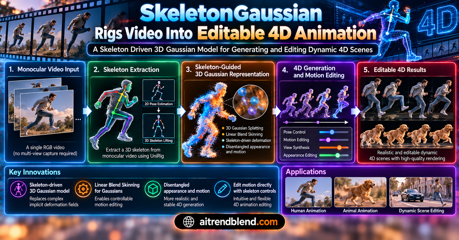
- SkeletonGaussian turns a single monocular video into a 3D Gaussian model driven by an extracted skeleton, rather than an opaque deformation field.
- Motion is split into two layers, large joint driven movement handled by linear blend skinning, and small residual detail handled by a lightweight hexplane and MLP.
- Because pose parameters grow only with the number of joints and frames, the method needs far less memory than dense deformation fields as sequences get longer.
- On the Consistent4D benchmark it reports a CLIP score of 0.923, an LPIPS of 0.125, and an FVD of 847.8, ahead of STAG4D, 4DGen, and DreamGaussian4D on all three.
- Editing a joint angle at one time step propagates the change through the whole clip, and the skeleton can be exported to tools such as Blender.
- The authors are candid that the approach struggles when an object has no clear skeletal structure, or when the skeleton extractor gets the topology wrong.
An animal you can pose is more useful than one you can only watch
Most work on generating dynamic 3D scenes treats motion as something to reconstruct, not something to control. A neural network watches a video, learns a warp field that explains how every point moved across every frame, and the result plays back like a recording. Want the deer to turn its head a bit further. Retrain the deformation field and hope. Want to pull the animation into Blender and add a second character. There is no rig to hand to the animator, only a dense field of numbers tied to a specific frame count.
SkeletonGaussian, described in a 2026 paper in Computational Visual Media by Lifan Wu, Ruijie Zhu, Yubo Ai, and Tianzhu Zhang, starts from a different assumption. Most objects that move, animals, robots, people, toys, already have an implicit skeleton, a set of rigid parts connected at joints. If a system can find that skeleton and use it to drive the bulk of the motion, then editing the motion becomes editing joint angles, which is a problem animators have solved for decades with tools like forward kinematics rigs. The paper frames its result plainly, calling the approach a new paradigm for controllable 4D generation, and the framing is worth taking seriously because the mechanism behind it is genuinely different from what came before.
Why deformation fields became the default, and what they cost
To see why this matters, it helps to know how the field got to implicit deformation fields in the first place. Text to 3D generation took off once score distillation sampling let researchers optimize a 3D representation using a 2D diffusion model as a critic, an idea introduced by DreamFusion and pushed further by DreamGaussian once Gaussian splatting arrived as a fast, differentiable alternative to neural radiance fields. Extending that idea to time added a fourth dimension, and the natural move was to let a neural field predict how each point in the scene shifts as a function of time, following the pattern set by dynamic NeRF work such as D NeRF and HexPlane.
That approach works, and it renders quickly once trained. But three practical problems follow directly from making the deformation implicit. Editing it usually means retraining, since the field has no meaningful internal structure a person can reach into. Its parameter count tends to grow with sequence length, so long clips become expensive to fit. And it produces nothing that standard animation software recognizes, no joints, no bones, no pose curves, just a function that happens to reproduce the video it was trained on. Sparse control point methods such as SC-GS and BAGS softened the first two problems by using a smaller set of control points instead of a dense field, but the control points still move according to a learned function rather than an explicit kinematic structure, so a user still cannot pose them the way an animator poses a rig.
Three stages, and a skeleton sitting in the middle
SkeletonGaussian’s pipeline runs in three stages, and the middle one is where the actual idea lives.
Stage one, build a static object and find its bones
The first stage picks the middle frame of the input video as a canonical reference, on the reasoning that the midpoint usually has the smallest average motion difference from every other frame, which keeps the rest of the pipeline stable. From that frame it optimizes a static 3D Gaussian model using a combination of multi view score distillation sampling and a photometric loss, the same basic recipe used by DreamGaussian style pipelines. Once the static Gaussian exists, the system extracts a mesh from it using an occupancy field and marching cubes, then hands that mesh to UniRig, a category agnostic rigging network, which proposes joints and their connectivity. A minimum spanning tree turns those candidate joints into an actual kinematic tree, the same kind of hierarchical bone structure a game engine or a 3D modeling tool would recognize.
Notice what this buys the pipeline early. Instead of inventing motion structure from scratch during training, the system borrows a rigging prior that was trained separately on a wide range of object categories, so it does not need to relearn what a joint even is for every new video.
Stage two, let the skeleton carry the big motion
Once joints exist, the paper applies linear blend skinning, the same technique behind SMPL for human bodies and SMAL for animals, to move the static Gaussian according to a learned pose sequence. Every joint gets a forward kinematics transform built by chaining together the local rotations of every ancestor joint in the tree, which is the standard way to compute where a hand ends up once you know how the shoulder, elbow, and wrist are all rotated.
Each Gaussian point then blends the transforms of its four nearest joints, weighted by inverse distance, which is a simple and training free way to decide how much influence a given joint has on a given piece of geometry.
The pose itself is stored as a tensor of quaternions, one per joint per frame, plus a single global translation for the root joint. That is a genuinely small amount of data compared to a dense deformation field, since it scales with the number of joints times the number of frames rather than growing with the complexity of the scene. The authors note that with roughly thirty joints and thirty two frames, the whole pose sequence for one object comes down to under three thousand scalar values, which is why the rigid stage alone needs the least memory and the shortest training time of any component in the system, according to their ablation numbers.
One detail worth flagging for anyone who wants to reproduce this. Optimizing raw per frame poses tends to overfit, chasing small tracking errors and producing a visible jitter in the joints. The fix here is a sliding window average across neighboring frames during training, smoothing each pose using its two nearest neighbors in time before it drives the skinning. It is a small addition, but the ablation table later in the paper shows it is not optional if you care about temporal quality.
Stage three, catch what the skeleton misses
A skeleton with thirty joints cannot represent a wrinkle in fabric or the subtle bunching of fur. For that, the paper freezes the skinning network and trains a separate refinement branch, a compact hexplane paired with a small MLP, that predicts a residual shift in position, rotation, and scale for each Gaussian, conditioned on the time index rather than directly on the pose. This is a deliberate two step training schedule, not a single joint optimization, and the ordering matters because it lets the skeleton settle on the coarse motion before the finer field is asked to clean up whatever is left.
The training signal across all three stages is the same combined objective, a multi view score distillation loss computed against anchor views generated by Zero123++, a photometric reconstruction loss against the reference frames, a foreground mask loss, and a regularization term on the refinement field to keep motion temporally smooth.
What the numbers actually say
The authors tested SkeletonGaussian against Consistent4D, STAG4D, 4DGen, and DreamGaussian4D on the Consistent4D benchmark, a set of twelve synthetic and twelve real world clips of thirty two frames each. Every method generates novel views from a frontal input video, and those renders get compared against ground truth footage using CLIP similarity, LPIPS perceptual distance, and FVD, which scores both frame quality and how consistent the motion looks over time.
| Method | CLIP ↑ | LPIPS ↓ | FVD ↓ |
|---|---|---|---|
| Consistent4D | 0.877 | 0.161 | 1518.5 |
| DreamGaussian4D | 0.913 | 0.143 | 994.1 |
| 4DGen (16 frames) | 0.909 | 0.137 | 913.1 |
| STAG4D | 0.909 | 0.126 | 992.2 |
| SkeletonGaussian | 0.923 | 0.125 | 847.8 |
The FVD gap is the number worth sitting with. A meaningfully lower FVD than every baseline points at fewer temporal artifacts frame to frame, which is exactly what you would hope an explicit kinematic structure would buy you over a field that has no concept of a rigid body moving through space.
The paper is refreshingly honest about the parts of its evaluation that are not conclusive. A blind pairwise user study with five participants across twenty video pairs found SkeletonGaussian preferred in fifty three of one hundred decisions against STAG4D, with both methods’ ninety five percent confidence intervals overlapping. The authors state directly that this result counts only as descriptive evidence, not a statistically significant win, which is the kind of admission you rarely see in a paper’s own results section and it earns the work some credibility precisely because of that restraint.
What the ablations reveal about where the quality comes from
Stripping the model down to just the rigid skeleton stage or just the non rigid hexplane stage shows the two halves are doing different jobs. Rigid only skinning keeps articulated structure intact but underfits fine motion, while non rigid only refinement improves per frame fidelity slightly yet loses temporal stability, since a field with no kinematic prior has no reason to keep a rigid limb rigid across frames.
| Configuration | CLIP ↑ | LPIPS ↓ | FVD ↓ | VRAM (MiB) ↓ | Training time ↓ |
|---|---|---|---|---|---|
| Rigid only (LBS) | 0.901 | 0.135 | 1012.6 | 0.01 | 12 min |
| Non rigid only (HexPlane and MLP) | 0.909 | 0.126 | 992.2 | 136.40 | 90 min |
| Full (rigid plus non rigid) | 0.923 | 0.125 | 847.8 | 136.41 | 102 min |
The memory line is the most telling number in the whole table. The rigid stage costs essentially nothing in VRAM because it only ever stores joint rotations, while the hexplane stage accounts for almost all of the memory footprint of the full system. Combining them barely changes memory use over the non rigid branch alone, which means SkeletonGaussian is not paying a heavy price for the added controllability it gets from the skeleton.
A second ablation swapped UniRig for Coverage Axis++, an older skeletonization method that selects points through coverage heuristics rather than a learned rigging prior. FVD rose from 847.8 to 890.4, and the paper reports that UniRig produces more stable, better aligned joints, which is a reminder that the whole system is only as good as the skeleton it starts from.
a new paradigm for controllable 4D generation Wu, Zhu, Ai, and Zhang, Computational Visual Media, 2026
The part that actually changes a workflow, editing after the fact
None of the quantitative gains would matter much if the skeleton were only an internal training scaffold. The reason this paper is worth a longer look is Section 3.5, where the authors describe a graphical interface for adjusting the poses of specific joints at specific time steps after the model has already been trained, with no retraining required. Because the kinematic tree is hierarchical, moving a parent joint automatically carries its children along with it, so rotating a shoulder moves the whole arm rather than leaving the forearm stranded in its old position. The resulting poses can be exported in standard skeleton and pose formats, which is what makes the Blender claim credible rather than aspirational, since most 3D software already knows how to read a bone hierarchy and a set of keyframed rotations.
Where the approach still runs into trouble
The authors are direct about the places this can fail, and it is worth taking them at their word rather than assuming the method is more general than it is.
- A skeleton extraction error, a joint placed in the wrong spot or connected to the wrong parent, propagates straight into the deformation and degrades the result. Objects without a clear articulated structure at all are explicitly called out as a case where the method performs poorly.
- The non rigid refinement branch is conditioned on time rather than on pose. That means when a user edits a skeleton pose, the coarse motion follows the edit correctly, but the fine grained residual detail stays tied to the original timeline, which can produce a visible mismatch for pose and time combinations the model never saw during training.
- Fixed inverse distance skinning weights, chosen because they need no training, can produce the classic candy wrapper artifact at joints with large rotation angles, a known failure mode of simple linear blend skinning that more sophisticated, learned skinning weight fields are built to avoid.
- The current system does not handle multiple independent objects in one scene, which limits it to single subject clips for now.
The paper also points toward where it goes next, including replacing the current pose optimization with initialization from a human pose estimator such as ViTPose for human centric clips, and connecting the extracted skeleton to ControlNet style conditioning so that a 3D skeleton could steer 2D video diffusion models directly, which would turn this from a standalone 4D pipeline into a component other generative systems could call on.
A reference implementation of the core idea
The paper does not release code alongside it, so the block below is our own from scratch PyTorch implementation of the mechanism it describes, built to make the moving parts concrete rather than to reproduce the authors’ exact training setup. It covers forward kinematics, inverse distance skinning weights, a small hexplane style residual field, the combined model, a simplified loss that swaps a synthetic multi view consistency term in place of an actual diffusion based SDS loss, a training loop, an evaluation pass, and a smoke test that runs on random data so you can confirm the shapes line up before pointing it at a real video.
Two honest caveats on the code above. The multi view consistency term is deliberately zeroed out and labeled as a proxy, because a faithful SDS loss needs a real diffusion model in the loop, which is outside the scope of a self contained demo. And the forward kinematics loop above runs per joint in plain Python for clarity, whereas a production system would vectorize that walk across the whole batch and joint tree at once for speed.
What this means beyond one deer and one toy robot
The most interesting part of this paper is not the benchmark numbers, it is the choice to treat a physically grounded structure as the main representation rather than as an afterthought bolted on for interpretability. That choice has a cost, since the system is only as reliable as the skeleton it extracts, and it clearly is not a fit for objects with no articulated structure at all, water, smoke, cloth without an underlying frame. But for the enormous category of things that do have joints, animals, robots, rigid tools, articulated furniture, it points toward 4D generation systems whose output plugs into the animation pipelines people already use, instead of output that has to be watched and never touched.
The authors also flag a natural next step that connects this work back to the broader generative video world, using the extracted 3D skeleton as a conditioning signal for 2D video diffusion models in the style of ControlNet or AnimateDiff. If that direction pans out, the skeleton stops being just an editing handle for one 4D asset and becomes a bridge between explicit 3D structure and the video generation models that currently have none.
Honest limitations, restated plainly
It is worth repeating the constraints in one place rather than letting them sit only inside a table. The method was evaluated on twenty four short clips, twelve synthetic and twelve real, each just thirty two frames long, so claims about long duration robustness go beyond what the paper actually tested. The user study behind the qualitative preference claim used five participants and one hundred pairwise judgments with overlapping confidence intervals, which the authors themselves say cannot support a claim of statistical significance. And two specific failure modes, skeleton topology errors and pose to time mismatch after editing, are acknowledged directly by the authors rather than left for a reader to discover independently, which is the kind of transparency that should be read as a point in the paper’s favor, not a weakness of the summary.
Conclusion
SkeletonGaussian’s core achievement is narrow and well defined. It takes a single monocular video, builds a static 3D Gaussian model, extracts a skeleton from that model using an existing category agnostic rigging network, and then splits all subsequent motion into a large, joint driven component handled by linear blend skinning and a small residual component handled by a lightweight hexplane field. That split is what lets the system beat four established baselines on CLIP, LPIPS, and FVD on the Consistent4D benchmark while using a fraction of the memory a dense deformation field would need for the same sequence length.
The conceptual shift matters more than any single number in the results table. Every recent 4D generation method before this one treated the deformation as something to be reconstructed as accurately as possible and then left alone. This paper treats the deformation as something a person should be able to reach into after training finishes, which changes what counts as a good result. A slightly less accurate reconstruction that exports a usable rig may be more valuable to an actual animator than a slightly more accurate reconstruction that cannot be touched.
Where this could travel next is fairly clear from the paper’s own future work section. Swapping in predefined templates like SMPL for human subjects, using pose estimators such as ViTPose to warm start the skeleton, and feeding the extracted 3D structure into video diffusion models as a control signal would all extend the same core idea, a skeleton as the primary control surface, into adjacent generation problems that currently lack anything like it.
The honest limitations are real and the authors do not dodge them. Objects without clear articulated structure are out of scope. Editing a pose after training currently produces a mismatch between the edited motion and the frozen, time conditioned residual detail. And a five person user study with overlapping confidence intervals is evidence, not proof, of a perceptual advantage over the strongest baseline tested. None of that undercuts the central contribution, it just marks where the next version of this idea needs to go.
What stays with you after reading the paper is not the FVD score. It is the image of an animator opening a generated deer, grabbing its foreleg, and simply moving it, the same way they would with any other rig, without retraining a single parameter.
Frequently asked questions
What does SkeletonGaussian actually take as input and produce as output
It takes a single monocular video of a moving object and produces a 3D Gaussian model driven by an explicit skeleton, along with a pose sequence for that skeleton and a small residual deformation field for fine detail such as clothing wrinkles.
How is this different from ordinary dynamic 3D Gaussian methods
Most dynamic 3D Gaussian methods learn an implicit deformation field that maps time to motion with no internal structure a person can edit. SkeletonGaussian instead extracts a real skeleton first and drives the bulk of the motion through that skeleton using linear blend skinning, so the motion has joints and poses rather than an opaque function.
Can the generated motion be edited after training finishes
Yes, and this is the paper’s main selling point. Users can adjust the pose of a specific joint at a specific time step through a graphical interface, and because the skeleton is hierarchical, moving a parent joint automatically carries its children along, with no retraining required.
Does the skeleton work with existing animation software such as Blender
The paper reports that the generated motion can be exported in standard skeleton and pose formats, which is what allows it to plug into ordinary 3D animation pipelines rather than staying locked inside the training framework.
What kinds of objects does the method struggle with
The authors are direct that objects without a clear articulated structure are a poor fit, and that errors in the automatic skeleton extraction step, wrong joint placement or wrong connectivity, propagate into the final motion and hurt quality.
Is there published code for SkeletonGaussian
[CODE REPOSITORY NEEDED, add a link once the authors release code or confirm none is planned]. The PyTorch example in this article is an independent illustration of the mechanism the paper describes, not the authors’ own implementation.
Read the full paper for the complete derivations, the ablation details, and the qualitative figures referenced above.
Read the paper (DOI)Related reading on this site
Wu, L., Zhu, R., Ai, Y., and Zhang, T. SkeletonGaussian, editable 4D generation through Gaussian skeletonization. Computational Visual Media, Vol. 12, No. 4, pages 925 to 939, August 2026. https://doi.org/10.26599/CVM.2026.9450557
This analysis is based on the published paper and an independent evaluation of its claims.