
Key points
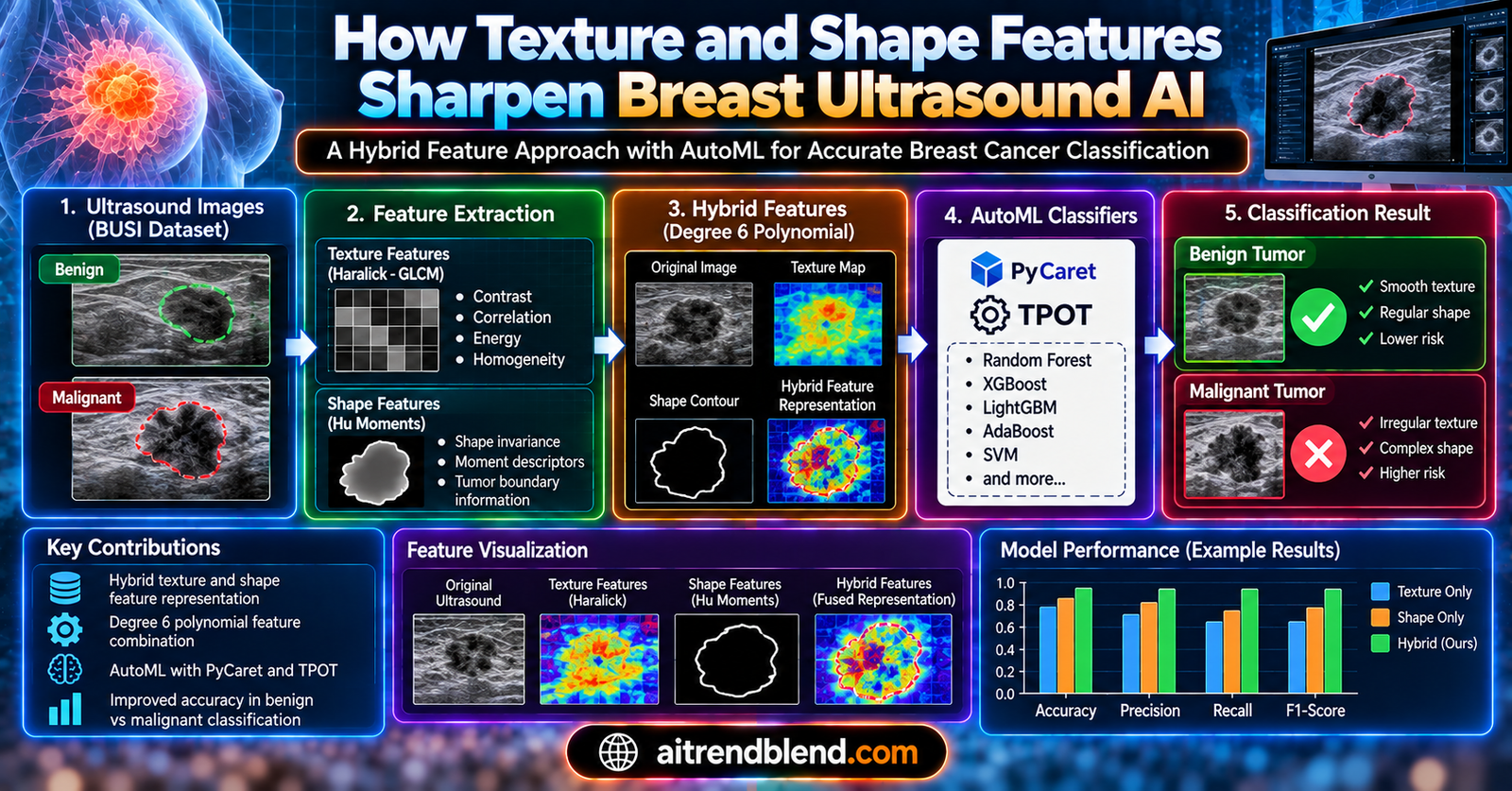
- The study builds six new hybrid features by folding Haralick texture measurements and Hu shape moments into a single degree six polynomial, rather than feeding texture and shape into a model as separate columns.
- Two AutoML systems, PyCaret and TPOT, independently searched among ten to fourteen classifiers each and both landed on the same hybrid feature as the strongest one.
- The winning feature, called y1 in the paper, pairs the energy value from the gray level co occurrence matrix with the first Hu moment, and reached 91.4 percent accuracy under PyCaret’s AdaBoost classifier.
- Three ensemble validation methods, bagging, boosting, and stacking, were run on top of the AutoML result, and stacking pushed the same feature to 92.8 percent under PyCaret and 92.2 percent under TPOT.
- The data comes from the public BUSI ultrasound archive, 487 benign and 210 malignant images, collected at a single hospital in Cairo, which matters for how far these numbers can travel.
The problem hiding inside a routine scan
Breast cancer statistics have a way of staying grim no matter how many times they get repeated. The World Health Organization logged over two million new cases worldwide in 2020 and close to seven hundred thousand deaths in the same year. In the United States alone, a quarter of a million new diagnoses were recorded in a single recent year. None of that is news to anyone who follows oncology research. What is less obvious is how much of the diagnostic process still depends on a trained eye reading a grainy grayscale image and making a judgment call.
Ultrasound remains one of the most accessible tools for a first look at a breast lesion, cheaper and faster than an MRI, and free of the radiation dose that comes with mammography. The tradeoff is that ultrasound images are noisy and operator dependent, and telling a benign fibroadenoma from an early malignant mass by eye is genuinely hard even for experienced radiologists. That is exactly the gap that computer aided diagnosis research has been chasing for two decades, and it is the gap this paper walks into.
Here is where it gets interesting. Most of the prior computer aided work reviewed by the authors picked one lane and stayed in it. Some studies pulled purely statistical features from the images. Others extracted textural descriptors from the gray level co occurrence matrix. A separate line of research focused only on geometric shape descriptors, the kind of measurements a radiologist would describe as well circumscribed versus ill defined borders. Very few studies tried to combine texture and shape into a single feature, and none, according to the literature review in this paper, tried to fuse them mathematically rather than just stacking them side by side in a feature table.
What earlier studies actually tried
The paper’s related work section is unusually candid about where earlier attempts fell short. Viswanath and colleagues built a computer aided diagnosis system using statistical features and three classifiers but never validated the result against a held out method. Kayode and colleagues extracted gray level co occurrence texture features for a support vector machine but worked with a small image set and no segmentation stage. Arefan’s team computed radiomic features from a region of interest marked by a radiologist and tested five classifiers, a more rigorous setup, but it came at a heavy computational cost. Sharma’s group and Ozcan’s group both explored geometric and anatomical features but left the hyperparameters at their defaults, a detail that sounds minor until you remember that an untuned classifier can leave real accuracy on the table.
A handful of more recent papers brought AutoML into the picture. Radzi’s team combined grid search with tree based AutoML and layered on ensemble methods for validation, closer in spirit to the present study. Rashed and colleagues went further and benchmarked seven different AutoML tools against eight datasets, a genuinely large effort, though it stayed limited to handcrafted anatomical features rather than anything texture based. What none of these prior efforts did, at least as far as this team could find after searching Google Scholar and PubMed, was fuse texture and shape into one engineered feature before handing it to a classifier. That absence is the opening the Galati team decided to fill.
Building a feature that behaves like a diagnosis
The core idea is worth sitting with for a moment because it is a little unusual. Instead of treating texture and shape as two separate inputs a classifier has to learn to weigh against each other, the authors pre combine them into a single number, once per lesion, using a fixed mathematical formula. The classifier never sees raw texture and raw shape. It only ever sees the fused result.
Isolating the lesion first
Before any feature gets computed, the team strips out everything in the ultrasound frame that is not the lesion itself. Each image in the BUSI dataset comes with a hand annotated binary mask marking the tumor boundary. The researchers overlay that mask on the original grayscale scan so that only the pixels belonging to the lesion remain, discarding the surrounding breast tissue, skin layer, and any text or markers burned into the image. This matters more than it might sound. A texture measurement computed across an entire ultrasound frame would be dominated by whatever fatty tissue or scanner artifacts happen to surround the tumor, not by the tumor’s own internal pattern. Cropping to the region of interest is what makes the later texture numbers actually mean something diagnostically.
Reading the texture with Haralick features
Once the lesion is isolated, the team computes six classic Haralick features from the gray level co occurrence matrix, a tool that has been part of the texture analysis toolkit since the 1970s. The six measurements are energy, entropy, homogeneity, contrast, correlation, and dissimilarity, and each one captures a different flavor of pixel arrangement.
Energy measures how uniform the pixel intensities are across the lesion, a smooth internal pattern produces a higher energy value. Entropy is close to the opposite idea, it rises when the pixel arrangement looks disordered and unpredictable. Homogeneity tracks how close together similar gray levels sit. Contrast and dissimilarity both grow when neighboring pixels differ sharply in intensity, which tends to happen around microcalcifications or irregular internal structure. Correlation captures how linearly related a pixel’s intensity is to its neighbor’s intensity. None of these six numbers alone tells a complete story, which is part of why the authors wanted to fold in shape information too.
Here \(p(i,j)\) is the probability that a pair of pixels at a fixed distance apart have gray level values \(i\) and \(j\), and \(N\) is the number of gray levels in the image. The remaining four Haralick measures, homogeneity, contrast, correlation, and dissimilarity, follow the same basic recipe, each weighting the co occurrence probabilities in a slightly different way depending on how far apart \(i\) and \(j\) sit.
Reading the shape with Hu moments
Shape gets a completely separate mathematical treatment. The binary mask, the same one used to crop the lesion, becomes the input for a set of Hu moments, a family of shape descriptors introduced back in the 1960s that stay stable no matter how a shape is rotated, scaled, moved, or mirrored. That stability matters clinically because a lesion photographed at a slightly different probe angle should not suddenly look like a different shape to the algorithm.
The authors lean on the clinical intuition that benign lesions tend to have smooth, well defined, roughly oval outlines, while malignant lesions often show jagged, poorly defined borders that spread irregularly into surrounding tissue. Hu moments are built to quantify exactly that kind of irregularity. The first Hu moment in particular relates closely to the overall area and spread of the shape, which the authors call out as the most clinically important of the seven.
where \(\mu_{pq}\) are the central moments of the binary shape, computed relative to its own centroid so that translation never affects the result. Four more moments follow the same pattern, each combining higher order central moments in a way that stays invariant under rotation and scaling.
Fusing the two with a polynomial, not an average
This is the part of the paper that separates it from most feature engineering papers, which usually just concatenate feature vectors and let the classifier sort out the relationships. Instead, the Galati team treats each Haralick feature as the input variable of a degree six polynomial, and treats the six Hu moments as the polynomial’s coefficients. Running one Haralick feature through this polynomial produces one hybrid feature, so six Haralick features paired with the same six Hu moment coefficients produce six hybrid features, labeled y1 through y6.
Why a polynomial instead of a straight average or a simple product. The authors argue that a linear combination would treat texture and shape as interchangeable, weighting them equally regardless of which one carries more diagnostic signal for a given lesion. A polynomial, by contrast, lets the higher order terms carry more weight from the earlier Hu moments, meaning the first moment, tied to lesion area and overall spread, dominates the result while later moments contribute smaller corrections. In effect, the shape information sets the scale of the response and the texture information determines how the curve unfolds across that scale. It is a clever way of saying that shape gets first say and texture gets to refine the answer, which lines up with how a radiologist actually reads a scan, glancing at the outline before scrutinizing internal texture.
Letting two AutoML systems argue it out
With six hybrid features computed for every one of the 697 usable images, benign and malignant only, normal cases from BUSI were dropped since there was no lesion to fuse features around, the team faced the usual next question in any machine learning pipeline. Which classifier, and with what settings, actually makes the most of this data.
Rather than hand pick a model and tune it by trial and error, which the authors point out is a genuinely inefficient process, they handed the labeled features to two different AutoML systems and let each one run its own search. PyCaret searched across fourteen candidate classifiers including LightGBM, gradient boosting, k nearest neighbors, AdaBoost, logistic regression, random forest, support vector machines, extra trees, decision trees, ridge classification, linear and quadratic discriminant analysis, and naive Bayes. TPOT took a different route entirely, using a genetic algorithm to evolve and recombine pipelines across eleven candidate classifiers including naive Bayes variants, decision trees, extra trees, random forest, gradient boosting, k nearest neighbors, support vector classification, logistic regression, XGBoost, and a multilayer perceptron.
The dataset was split so that seventy percent of the images fed training and thirty percent were held back for testing, a fairly standard split, and each of the six hybrid features was run through both AutoML systems independently, six features times two systems, twelve separate searches in total.
The numbers that came back
Both systems converged on the same answer even though they searched completely different spaces of models. y1, the fusion of energy and the first Hu moment, came out on top under both AutoML tools.
| Feature | PyCaret best model | PyCaret accuracy | TPOT best model | TPOT accuracy |
|---|---|---|---|---|
| y1 (energy) | AdaBoost | 0.914 | Multilayer perceptron | 0.906 |
| y2 (entropy) | AdaBoost | 0.895 | Decision tree | 0.894 |
| y3 (homogeneity) | Logistic regression | 0.763 | Naive Bayes | 0.759 |
| y4 (contrast) | Gradient boosting | 0.784 | K nearest neighbors | 0.772 |
| y5 (correlation) | Logistic regression | 0.821 | Naive Bayes | 0.809 |
| y6 (dissimilarity) | Logistic regression | 0.788 | K nearest neighbors | 0.759 |
For the winning feature, PyCaret’s AdaBoost model reached an AUC of 0.955, recall of 0.919, precision of 0.895, an F1 score of 0.907, and a Matthews correlation coefficient of 0.826. TPOT’s multilayer perceptron, tuned to a learning rate of 0.5 and default regularization, reached a higher AUC of 0.981 but a lower recall of 0.850, with an F1 score of 0.901 and an MCC of 0.818. Interestingly the two systems traded strengths, PyCaret caught more true malignant cases while TPOT’s ranking of predictions was slightly more separable overall. Neither model dominates the other cleanly, and reporting both, rather than only the flattering one, is one of the more honest choices in this paper.
The remaining four features, y3 through y6, all landed in the 0.76 to 0.82 accuracy range, noticeably behind y1 and y2. The authors trace this gap back to the violin plots they ran before classification even started. For y1 and y2, benign and malignant scores clustered around clearly separated medians, 0.18 versus 0.14 and similar values. For y3 through y6, the distributions looked chaotic and overlapping between classes, which the paper is refreshingly willing to describe as a loss of information rather than dressing it up as a modeling limitation.
Checking the answer with three different validation methods
A classifier chosen by an AutoML search can still be an accident of a particular test split, so the team ran three ensemble validation techniques on top of the AutoML result, each computed with ten fold cross validation to guard against overfitting on any single partition of the data.
| Validation method | PyCaret features, y1 accuracy | TPOT features, y1 accuracy |
|---|---|---|
| Bagging | 0.921 | 0.912 |
| Boosting | 0.901 | 0.900 |
| Stacking | 0.928 | 0.922 |
Bagging trains many copies of a k nearest neighbors classifier on bootstrapped subsets of the training data and averages their votes, which tends to reduce the variance that comes from any one unlucky training split. Boosting, using XGBoost in this study, trains classifiers sequentially, with each new one focused on correcting the mistakes of the last. Stacking, the method that performed best across the board, trains a logistic regression and random forest as base models and then uses a support vector regression as a meta learner to combine their predictions.
Where this sits against other AutoML studies
The paper closes its results section with a comparison table pulling in five other AutoML based breast cancer studies from the last five years. Labilloy’s team, using PyCaret on care adherence data rather than image features, reached only 0.63 AUC. Sihombing’s group hit 0.85 accuracy with a PyCaret random forest on anatomical features. Zhuang’s genetic and clinical feature study landed at 0.763 accuracy with LightGBM. Rashed’s TPOT XGBoost pipeline on anatomical features reached 0.912 accuracy, close to this paper’s own result. Wan’s AutoML Vision comparison against a random forest baseline reported 0.91 accuracy and an 0.87 F1 score on ultrasound lesion classification directly.
Set against that field, the hybrid feature approach’s 0.914 accuracy under PyCaret and 0.906 under TPOT sit near the top of the comparison table, and the 0.955 to 0.981 AUC range is higher than anything else listed. None of the comparison studies fused texture and shape mathematically the way this one does, which makes a direct apples to apples comparison a little unfair in both directions, but the numbers at least suggest the hybrid feature idea is not losing anything by trading two feature types for one engineered one.
Clinical translation gap
It is worth being blunt about the distance between a strong accuracy number in a paper and something a hospital could actually deploy. This model was trained and tested entirely on one public archive, BUSI, built from patients at a single hospital in Cairo using presumably a consistent scanner and imaging protocol. Real world deployment would mean different ultrasound machines, different probe frequencies, different operator habits, and patient populations with different breast densities and demographics, all factors known to shift how texture and shape features behave. Nothing in this paper tests that kind of cross site generalization, and the authors do not claim otherwise.
There is also the practical matter of segmentation. Every hybrid feature in this study depends on an accurate lesion mask. The BUSI masks were presumably drawn by trained annotators under relatively controlled conditions. An automated segmentation step in a live clinical pipeline, run on noisier real world images, would introduce its own error that could ripple straight through into the hybrid feature calculation and, from there, into the final classification. A method this sensitive to mask quality needs a validated automatic segmentation stage before it could reasonably sit in a real diagnostic workflow, and building one was explicitly left for future work.
Reading the honest limitations
To their credit, the authors do not hide behind their accuracy numbers. They flag image quality, the choice of segmentation method for the ground truth masks, and the total number of images as direct limitations on how far the results generalize. The dataset itself is modest by deep learning standards, 487 benign and 210 malignant images, which is workable for classical machine learning on engineered features but would be considered small for training a convolutional network from scratch.
There is also a subtler limitation buried in the discussion section. The authors note that malignant and benign lesions in this dataset sometimes share very similar geometric shapes, which they suggest is a real source of the misclassifications seen across all six features, not just the weaker ones. If shape overlap between classes is a genuine feature of the underlying biology and not just an artifact of this particular dataset, then Hu moments alone, or fused with any texture measure, may have a hard ceiling they cannot easily push past no matter how the polynomial is tuned.
Finally, only benign and malignant classes were used, with the 133 normal cases in BUSI excluded entirely because the hybrid features require a lesion mask to compute shape descriptors from. That is a reasonable methodological choice given how the features are built, but it does mean this particular pipeline, as published, cannot yet distinguish a lesion from no lesion at all, only classify a lesion once one has already been identified and segmented.
Trying it yourself, a PyTorch walkthrough
The original paper implements its classifiers in scikit learn through PyCaret and TPOT rather than in PyTorch. The code below reconstructs the same pipeline in PyTorch so you can see the moving parts end to end, from raw texture and shape computation through the polynomial fusion step and into a neural classifier modeled on the multilayer perceptron TPOT selected for the winning feature. It runs on synthetic data out of the box so you can confirm the pipeline works before pointing it at your own segmented ultrasound images.
Swap the synthetic data generation block for real Haralick and Hu moment values pulled from your own segmented ultrasound archive, using the functions above, and this becomes a working reproduction of the paper’s y1 pipeline through to a trainable classifier. The genetic search TPOT ran internally and the hyperparameter tuning PyCaret performs are both simplified here into a fixed architecture and a standard Adam optimizer, which will not match the original accuracy numbers exactly but demonstrates the same fusion logic end to end.
What this means beyond one dataset
Set aside the specific accuracy numbers for a moment and look at the underlying idea. Fusing two categories of handcrafted features through a fixed mathematical operation, rather than concatenating them and hoping a classifier learns the relationship, is a strategy that could travel well beyond breast ultrasound. Any imaging task where both the internal texture of a region and its outer shape carry diagnostic weight, thyroid nodules, skin lesions, certain lung nodules on CT, could in principle be approached the same way, provided a reliable segmentation mask is available to compute the shape half of the equation.
The choice to validate the AutoML result with three separate ensemble methods also deserves attention as a general practice, not just a footnote in this particular paper. A lot of published machine learning work in medical imaging reports a single accuracy number from a single train test split and calls it a day. Running bagging, boosting, and stacking on top of an AutoML selected model, each with its own ten fold cross validation, gives a far more honest picture of how stable that accuracy number actually is. The fact that stacking consistently outperformed the raw AutoML result across nearly every feature in this study is itself a useful finding independent of the specific hybrid feature idea.
Limitations worth repeating before anyone gets excited
None of the enthusiasm above should obscure how early stage this work still is. A single public dataset from a single hospital, 697 usable images total, a hand annotated segmentation step that has not been automated or validated at scale, and no external test set from a different clinic or scanner all mean this is a promising proof of concept rather than anything close to a deployable diagnostic aid. The authors themselves frame it that way in their conclusion, pointing toward future work on fractal dimension features and toward combining handcrafted features like these with deep learned ones, rather than claiming the current pipeline is finished.
There is also a quieter methodological question the paper does not fully resolve. Feeding a single scalar hybrid feature into a classifier, one number per lesion, discards a lot of information that six separate raw features, or a full deep feature vector, would retain. The fact that y1 alone reaches 91.4 percent accuracy is genuinely impressive for a single number, but it also raises the question of how much further accuracy might be available by combining y1 with y2, or by feeding all six hybrid features into a classifier together rather than evaluating each one in isolation. That combination was not tested here and stands out as an obvious next experiment.
Conclusion
What this paper ultimately demonstrates is that a fairly old idea, the gray level co occurrence matrix, and an even older one, Hu’s invariant shape moments, still have room to produce something new when combined in a deliberate mathematical way rather than simply placed side by side in a feature table. The degree six polynomial fusion is a small piece of algebra, but it encodes a real clinical intuition, that shape sets the frame a radiologist reads a lesion within and texture fills in the details inside that frame.
The conceptual shift here is subtle but important for anyone building feature based diagnostic tools rather than end to end deep networks. Instead of asking a classifier to discover the relationship between two feature families on its own, the authors baked a specific, interpretable relationship into the feature itself before the classifier ever saw it. That trades some flexibility for a large gain in interpretability, since a clinician or a downstream researcher can trace exactly how the first Hu moment and the energy value combine to produce the number the AdaBoost model is actually classifying, something that is much harder to say about a deep convolutional feature vector.
Whether this specific fusion strategy generalizes to other cancer types or other imaging modalities is an open question the authors themselves flag as future work. Thyroid ultrasound, skin lesion photography, and even certain CT based lung nodule tasks share the same basic structure of an internal texture pattern wrapped inside a diagnostically meaningful outer shape, and the polynomial fusion idea does not appear to depend on anything unique to breast tissue specifically.
The honest limitations matter as much as the headline accuracy number. A single hospital’s dataset, a hand drawn segmentation mask, and no external validation cohort mean this result needs to be reproduced on independent data before anyone starts talking about clinical translation. The authors’ own next steps, adding fractal dimension features and exploring hybrids of handcrafted and deep learned representations, suggest they see this paper as one step in a longer research program rather than a finished tool.
If nothing else, this study is a useful reminder that the newest deep learning architecture is not the only path to a meaningful gain in medical image classification. Sometimes the more interesting move is figuring out a smarter way to combine the tools that have been sitting on the shelf for fifty years.
Frequently asked questions
What is a hybrid feature in this study, in plain terms
It is a single number computed for each breast lesion that blends how rough or smooth the internal tissue looks, called a Haralick texture feature, with how regular or irregular the lesion’s outline is, called a Hu moment. The two are combined using a degree six polynomial rather than simply averaged.
Which hybrid feature performed best and why
The feature called y1, built from the energy Haralick measurement and the first Hu moment, performed best under both AutoML systems tested. The authors attribute this to a clean separation between benign and malignant score distributions for that particular feature, visible in their violin plots, compared with the more overlapping distributions seen for the other five features.
What accuracy did the study achieve
PyCaret’s AdaBoost classifier reached 91.4 percent accuracy on the y1 feature, and TPOT’s multilayer perceptron reached 90.6 percent on the same feature. After stacking based ensemble validation with ten fold cross validation, those numbers rose to 92.8 percent and 92.2 percent respectively.
What dataset was used and how large is it
The study uses the public Breast Ultrasound Images Dataset, known as BUSI, collected from 600 patients at Baheya Hospital in Cairo. Only the 487 benign and 210 malignant images were used, since the hybrid features require a lesion mask that the 133 normal images do not have.
Is this method ready to be used in a hospital
No. It was trained and tested on a single public archive from one hospital, relies on hand drawn segmentation masks rather than an automated segmentation step, and has not been validated on an independent dataset from a different clinic or scanner. The authors present it as a research contribution, not a clinical tool.
How does this compare with other AutoML studies on breast cancer
Against five other AutoML based studies from the last five years cited in the paper, ranging from 0.63 to 0.91 in reported accuracy or AUC depending on the metric used, this study’s 0.914 accuracy and 0.955 to 0.981 AUC range sit at or near the top, though the comparison studies used different feature types, mostly anatomical or clinical rather than image texture and shape.
Read the full open access paper, including all six equations for the Haralick features and Hu moments, at Scientific Reports.
Read the paper Get the BUSI datasetThe full source paper, including every equation referenced above, the complete list of prior studies compared in Table 1, and the violin plots for all six hybrid features, is available through its DOI at doi.org/10.1038/s41598-025-09554-2. The generated hybrid feature dataset behind this study’s tables is also hosted publicly on the authors’ GitHub repository.
Tabacaru, G., Moldovanu, S., Munteanu, D. and Barbu, M. New hybrid features extracted from US images for breast cancer classification. Scientific Reports 15, 25690 (2025). This analysis is based on the published paper and an independent evaluation of its claims.