
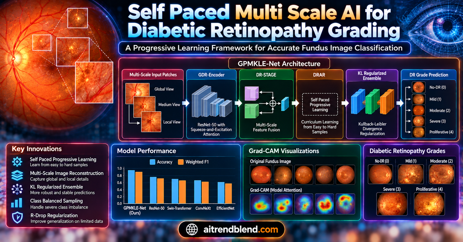
Key points
- The proposed network, called GPMKLE-Net, reached an AUC of 0.9907 on a combined Messidor and Kaggle dataset, a 2.2 percent gain in AUC over a plain ResNet-50 baseline.
- Training starts on shuffled small patches of the fundus image and gradually moves to the full picture, a curriculum the authors call randomized multi scale image reconstruction.
- A class balanced focal loss and a histogram based resampling step target the chronic shortage of Mild grade examples in public diabetic retinopathy datasets.
- An R-Drop style consistency term pulls the predictions of parallel classifier heads into agreement, which the ablation table shows adds real accuracy on top of the other two ideas.
- Recall for the No-DR class reached 97.65 percent and recall for the Severe class reached 98.55 percent, with precision above 91 percent in every category on the four class task.
- The authors are candid that separating Mild from Moderate disease remains hard and that the model does not yet localize individual lesions.
This article explains a piece of published research. It is not medical advice, diagnosis, or treatment.
Nothing here should be used to make decisions about your own eye care or anyone else’s. If you have diabetes or are concerned about your vision, talk with an ophthalmologist or another qualified eye care professional.
Why grading diabetic retinopathy is harder than it sounds
Diabetic retinopathy is a complication of diabetes that damages the small blood vessels feeding the retina. The scale of the problem is large and growing. The paper cites International Diabetes Federation figures showing roughly 463 million people living with diabetes worldwide in 2019, a number that had already climbed to an estimated 537 million by 2021, with a projection of 783 million by 2045. Global prevalence of diabetic retinopathy among people with diabetes is put at 34.6 percent, which means the eye exam described at the top of this article is not a rare event. It happens millions of times a year.
The clinical challenge is that the earliest damage is small on purpose, in the sense that the disease starts with microaneurysms, tiny bulges in the retinal capillaries that can be smaller than 125 micrometers across. A human grader working through a stack of fundus photos can miss these, especially in borderline cases where an eye sits right at the line between Mild and Moderate disease. Automated grading promises consistency and scale, yet the datasets used to train such systems tend to be small relative to other computer vision tasks, unevenly split across severity grades, and collected on different cameras with different color casts and exposure levels. A model trained on this kind of data can look strong on paper and still stumble on a doctor’s actual patient population.
What earlier deep learning approaches got right, and where they ran short
Convolutional networks have already shown they can match expert level performance on several medical imaging tasks, from lesion detection to full disease grading. The paper’s related work section points to a common thread across that literature. Image preprocessing choices matter a great deal, and the authors reference work by Lam and colleagues showing that a method as simple as adaptive histogram equalization can help in some settings and actively hurt others once the task becomes multi class rather than binary. Other groups have chased accuracy through architectural complexity, combining multi scale filtering with residual connections, an approach explored by Gangwar and Ravi, or by stacking several models into an ensemble. Ensembles do tend to raise accuracy, but the paper is upfront that they come with a real computational cost, and that cost only grows as more models join the vote.
None of that fully solves the underlying data problem. Small, imbalanced training sets push conventional convolutional networks toward two failure modes at once. They overfit to the majority classes because that is where most of the gradient signal comes from, and they underfit the rare classes because there simply are not enough examples to learn a stable representation. Heavier ensembles do not fix this tension, they just spread the same weak signal across more parameters. The authors frame their contribution as a way to get more out of a single backbone network rather than reaching for a bigger one.
The architecture, piece by piece
The full system is named GPMKLE-Net, short for Guided Progressive Multi-scale KL-Ensemble Network. It is built around a ResNet-50 backbone pretrained on ImageNet, modified so that feature maps from its final three stages are pulled out separately rather than only using the last layer’s output. Three ideas sit on top of that backbone, and each earns its own subsection in the paper.
The DRAR block adds attention without losing shallow detail
The authors note that shallow layers in a convolutional network are good at capturing texture and shape, while deeper layers trade that spatial detail for more abstract representations. To keep some of that shallow sensitivity available deeper in the network, they augment the backbone’s residual blocks with a Squeeze-and-Excitation attention mechanism, forming what they call a Diabetic Retinopathy Attention Residual block, or DRAR. Squeeze-and-Excitation works by pooling each feature channel down to a single number with global average pooling, passing that vector through a small fully connected network, and using the result to reweight the original channels. In effect the network learns which feature channels matter most for a given image and turns up their volume. Combined with multi scale convolution inside the same block, the DRAR module is meant to help the network zero in on pathological texture, the kind of subtle mottling and small vessel change that marks early disease.
The GDR-Encoder and GDRC fuse information across depth
Features pulled from different depths of the backbone do not automatically talk to each other, so the paper introduces a Guided Diabetic Retinopathy Encoder, GDR-Encoder for short, that reprocesses each stage’s output through paired convolution, batch norm, and ReLU blocks followed by max pooling. The re-encoded features from multiple stages are then concatenated and passed into the Guided Diabetic Retinopathy Classifier, or GDRC, which is a multilayer perceptron that uses dropout in a way borrowed from R-Drop, a regularization technique published by Wu and colleagues in 2021. Two forward passes through the same dropout-equipped classifier produce two slightly different probability distributions over the four or five severity classes, and the network is pushed to keep those two distributions close to each other. The practical effect is a kind of built in ensemble, since each dropout mask behaves like a slightly different sub model, and forcing agreement between them tends to make the final prediction more stable.
An ensemble classification head votes across stages
The final piece treats each of the three backbone stages, plus the fused concatenation stage, as an approximate sub model in its own right. Each of the four produces its own prediction for the input image, and a voting scheme combines them into the final classification. This is a lighter weight version of the ensemble idea than training four full separate networks, since the four heads share almost all of their parameters through the shared backbone, yet it still gives the model several independent opinions to draw on before committing to a grade.
Guided progressive multi scale learning, the curriculum that gives the network its name
The most distinctive part of the paper is not a new layer type, it is a training curriculum the authors call Guided Progressive Multi-scale Learning, or GPML. The idea borrows from self paced learning, a meta learning concept where a model is deliberately shown easier examples first and harder ones later, and pairs it with a jigsaw style image reconstruction step adapted from work by Du and colleagues on fine grained visual classification.
Here is how the curriculum unfolds across four training steps, all applied to the same batch of 224 by 224 pixel fundus images. In step one, each image is cut into 64 small patches, each 28 by 28 pixels, which are shuffled and reassembled into a scrambled version of the original photo. In step two, the patch count drops to 16, each 56 by 56 pixels, giving the network somewhat larger, less scrambled chunks to work with. Step three uses just 4 patches at 112 by 112 pixels each. Step four presents the full, unscrambled 224 by 224 image. Each step has its own loss signal, and features from the first three steps pass through their own deep feature encoders before being fused together in step four through a module the paper calls Multi-level Feature Fusion.
The logic mirrors how a person might first notice scattered flecks of discoloration across a photo before recognizing them as a coherent lesion once the full picture comes into view. Grad-CAM style heatmaps included in the paper back this up visually. In the earliest training stage, the network’s attention is scattered across many regions of the image, consistent with it hunting for any locally unusual texture. As training and network depth progress, attention consolidates onto more coherent, clinically relevant regions, and in one moderate grade example the authors highlight, the model’s later stage attention lands squarely on a yellow white hard exudate, a recognizable diabetic retinopathy lesion.
The loss function that ties it together
GPMKLE-Net is trained with a composite objective that sums three separate loss terms, each solving a different piece of the puzzle.
Ordinary cross entropy loss, written as L_CE, does the baseline job of pushing predicted class probabilities toward the ground truth label. On its own it tends to be dominated by whichever class has the most examples, which is where the second term comes in.
This is a class balanced loss with focal weighting, adapted from Cui and colleagues’ 2019 work on effective sample number weighting combined with the focal loss idea of down weighting easy examples. Here C is the number of severity classes, n_y is the number of training samples in the target class, and β is a tunable value that controls how strongly rare classes get boosted. The focal term (1 - p_j^t)^γ further sharpens the model’s attention onto samples it is currently misclassifying, rather than spending capacity on cases it already gets right.
This is the R-Drop term, a symmetric Kullback-Leibler divergence between the output distributions p and q produced by two dropout passes through the GDRC classifier. Minimizing it discourages the network from relying on any single random dropout pattern and, according to the paper’s ablation results discussed below, meaningfully improves stability.
The three terms are combined with tunable weights λ_CE, λ_CB, and λ_Rdrop, giving the authors a knob to balance raw classification accuracy against class fairness and prediction consistency.
Cleaning up and balancing the data before any of this can work
No amount of clever architecture rescues a model trained on messy, lopsided data, and the paper spends real effort on preprocessing. Images pass through Otsu thresholding, a classic method for separating the round retinal image from its black surrounding border, which reduces the chance that the model wastes capacity learning artifacts of dark corners rather than the eye itself. Color standardization follows, normalizing each RGB channel’s pixel intensities against the dataset’s overall mean and standard deviation, which helps offset the fact that fundus photos in these public datasets come from different cameras and clinics with visibly different color casts.
Class imbalance gets its own dedicated fix. The authors use what they call Histogram Equalization Sampling, HES for short, which adjusts both the sampling weight and the effective quantity of each class during training so that underrepresented grades are not quietly ignored. This sampling strategy works alongside the class balanced focal loss described above rather than replacing it, and the paper credits the pairing with a clear jump in the model’s ability to tell Mild disease apart from its neighbors, a distinction that has historically been one of the weakest points for automated graders.
Where the images came from
The core training and evaluation set combines Messidor-1, a French government funded dataset of 1200 carefully annotated fundus images collected across three ophthalmology facilities, with a targeted addition of 125 high quality Mild grade images pulled from the much larger 2015 Kaggle Diabetic Retinopathy Detection dataset. The result, which the paper refers to as the MESSIDOR-Kaggle dataset, contains 546 Normal, 278 Mild, 247 Moderate, and 254 Severe images for 1325 total, split 70 percent for training and 30 percent held out for validation and testing. The APTOS 2019 Blindness Detection dataset, with 3662 images across five severity grades, is used as a separate resource to check how well the approach generalizes beyond the primary training mix.
| Dataset | Normal / No-DR | Mild | Moderate | Severe | Proliferative | Total |
|---|---|---|---|---|---|---|
| Kaggle DR (source pool) | 25810 | 2443 | 5292 | 873 | 708 | 35126 |
| APTOS (validation set) | 1805 | 370 | 999 | 193 | 295 | 3662 |
| Messidor-1 (core set) | 546 | 153 | 247 | 254 | — | 1200 |
| MESSIDOR-Kaggle (training mix) | 546 | 278 | 247 | 254 | — | 1325 |
Training itself ran for 300 epochs using stochastic gradient descent with a batch size of 32, a weight decay of 5 × 10^-4, and momentum of 0.9. The starting learning rate of 8 × 10^-3 followed a cosine annealing schedule down to a floor of 1 × 10^-5. Standard augmentations were applied during training, including resizing, center and random cropping to 224 by 224 pixels, horizontal flips with 0.5 probability, and random rotations up to 90 degrees. All experiments ran in PyTorch on an NVIDIA A5000 GPU.
How well did it actually work
On the combined MESSIDOR-Kaggle four class task, GPMKLE-Net reached 94.47 percent accuracy and an AUC of 0.9907, ahead of every comparison method the authors tested, including recent transformer and hybrid architectures.
| Method | Accuracy | AUC |
|---|---|---|
| ViT | 67.34% | 0.8597 |
| Swin-Transformer | 73.87% | 0.8900 |
| MobileNet-V3 | 80.15% | 0.9356 |
| DCT-ResNet50 | 86.68% | 0.9636 |
| HRNet | 87.44% | 0.8982 |
| Xception | 89.20% | 0.9558 |
| ResNeXt | 91.96% | 0.9794 |
| GoogleNet | 92.21% | 0.9735 |
| ResNet-50 (baseline) | 92.71% | 0.9687 |
| ConvNeXt | 92.71% | 0.9721 |
| GPMKLE-Net (proposed) | 94.47% | 0.9907 |
Per class figures tell a more clinically relevant story than the accuracy headline. In the final model, No-DR recall reached 97.65 percent with precision of 96.54 percent, meaning the network rarely missed a genuinely healthy eye and rarely flagged one incorrectly. Severe disease recall reached 98.55 percent, an important number since missing a Severe case carries real consequences for a patient’s care pathway. Precision stayed above 91 percent in every one of the four categories. The Mild class, historically the weak point for this task, reached 92.93 percent recall and 91.66 percent precision in the full model, a marked improvement over the plain ResNet-50 baseline’s 85.99 percent recall for that same class.
On the separate APTOS validation set, using a five class grading scheme, GPMKLE-Net posted the highest AUC among all compared methods at 0.9872, ahead of Swin-Transformer, ViT, and ConvNeXt on that metric. Its raw accuracy of 93.45 percent came in slightly below ConvNeXt’s 94.90 percent, which the authors read honestly, noting that GPMKLE-Net separates classes more reliably across the full range of decision thresholds while ConvNeXt edges it out on point accuracy for individual samples.
The ablation table shows each idea earning its keep
Rather than presenting the full system as a black box, the paper breaks down what each addition contributes on top of a plain ResNet-50 baseline.
| Configuration | Accuracy | AUC | Severe recall | Severe precision |
|---|---|---|---|---|
| ResNet-50 baseline | 92.71% | 0.9687 | 93.30% | 92.09% |
| + RMIR (multi scale curriculum) | 93.22% | 0.9801 | 97.24% | 91.25% |
| + RMIR + HES (balanced sampling) | 93.97% | 0.9850 | 98.55% | 94.82% |
| + RMIR + HES + GLL (full guided loss) | 94.47% | 0.9907 | 98.55% | 92.48% |
Adding the randomized multi scale curriculum by itself pushed AUC from 0.9687 to 0.9801 and lifted Severe class recall by close to four points, although it did trade away some Moderate class recall along the way, a reminder that no single change is free of tradeoffs. Layering in the histogram equalization sampling on top of that recovered ground on the Moderate class and pushed Mild class recall from 85.99 to 88.77 percent, with the paper’s confusion matrix analysis showing a genuinely reduced rate of Mild versus Moderate mix ups, the specific confusion that clinicians and prior automated systems both struggle with. Finally, adding the guided loss combination, cross entropy plus the class balanced focal term plus R-Drop consistency, brought the final jump to 94.47 percent accuracy and 0.9907 AUC, with a large boost to Mild class precision that lands the full model at 91.66 percent for that category.
The scarcity of Mild grade images is not a minor data quality footnote, it is the reason automated diabetic retinopathy grading has struggled at the exact severity boundary where early intervention matters most. Reading of the paper’s discussion of class imbalance and the Mild category
What the confusion matrix reveals
The paper includes confusion matrices for GPMKLE-Net alongside HRNet, Swin-Transformer, and ViT on the same four class test split. GPMKLE-Net’s matrix is heavily diagonal, with 170 of 174 true No-DR cases correctly classified, 67 of 72 Mild cases correct, 64 of 76 Moderate cases correct, and 75 of 76 Severe cases correct. The comparison methods show noticeably more off diagonal spread, particularly ViT, which misclassified a meaningful share of No-DR cases as Moderate or Severe, an error pattern that would be far more consequential in a clinical setting than the reverse.
The clinical translation gap
A strong AUC on a held out split of 1325 curated images is not the same thing as a system ready to sit inside a screening workflow. Messidor-1’s images came from three ophthalmology facilities under a coordinated collection protocol, and the added Mild images and the APTOS validation set bring in Kaggle sourced photos captured on varying equipment. That mix helps the model see more visual diversity than a single site dataset would offer, yet it still falls well short of the range of cameras, lighting, patient demographics, and comorbid eye conditions a system would meet in routine screening across many clinics and countries. The paper’s own validation strategy, training and testing on a 1325 image core set with APTOS held out separately, is a reasonable academic setup, but it does not stand in for a prospective clinical trial with a defined patient population and a comparison against practicing graders working under real time constraints.
There is also a gap between grading severity and guiding care. GPMKLE-Net assigns a class label to a whole image. It does not, in this version, draw a box around the microaneurysm or hard exudate driving that label, something the authors flag directly as future work. A clinician using a tool like this would still need some way to see which region of the retina triggered a given grade before trusting it in a diagnostic pathway, particularly for a Severe classification that might prompt an urgent referral.
Honest limitations, in the authors’ own words and in the numbers
The discussion section of the paper is refreshingly direct about what has not been shown. Three limitations stand out.
First, generalizability has not been established beyond the datasets used here. The core training and test set totals 1325 images, and while APTOS adds another 3662 for validation, both sources trace back to a small number of collection efforts rather than a broad, multi country clinical sample. A model that performs at 0.9907 AUC on this mix could see that number move once it meets cameras, populations, and disease severity distributions it has never encountered.
Second, Mild versus Moderate separation remains the model’s weakest link even after every improvement in the paper. The ablation table’s own numbers show Moderate class recall topping out at 88.77 percent under the RMIR plus HES configuration and settling at 84.10 percent in the full guided loss model, notably lower than every other class’s recall figure. That is the clinically important edge case, the one where a wrong call in either direction changes a patient’s follow up schedule.
Third, the paper does not attempt lesion level localization. Grad-CAM heatmaps offer a qualitative look at where the network’s attention lands, and the authors’ own moderate grade example nicely highlights a hard exudate, but that is a visualization tool for researchers, not a bounding box or segmentation mask a clinician could act on directly. The authors list expanding and diversifying the training data, sharpening feature extraction for subtle cases, and building in explicit lesion localization as their stated next steps, alongside exploring self supervised and unsupervised pretraining and transfer learning from adjacent medical imaging tasks.
Where this fits in the broader push toward automated eye screening
The specific numbers in this paper matter less on their own than the pattern they illustrate. A recurring theme across recent diabetic retinopathy research, and across medical imaging more broadly, is that architecture alone rarely closes the gap between a research benchmark and a clinically trustworthy tool. Data curation choices, training curricula that respect how hard different examples are, and honest treatment of class imbalance keep showing up as the levers that move real world performance, often more than swapping in a fancier backbone network. GPMKLE-Net’s central move, teaching a fairly ordinary ResNet-50 to look at scrambled patches before it looks at the whole photo, is a specific instance of a general idea that keeps resurfacing in low data medical imaging work, that a well designed curriculum can substitute for data volume the field simply does not have.
That said, the gap between a strong AUC on a curated academic dataset and a system deployed inside a screening program remains wide, and this paper is candid about sitting on the research side of that gap. Readers evaluating any diabetic retinopathy AI tool, whether this one or a commercial product built on similar ideas, should look for prospective validation on a population resembling the one it will actually serve, clear reporting of per class performance rather than a single headline accuracy figure, and some mechanism for showing clinicians where in the image a flagged finding actually sits.
Conclusion
GPMKLE-Net earns its place in the diabetic retinopathy literature not because it introduces an exotic new architecture, but because it takes a familiar ResNet-50 backbone and asks a genuinely useful question, how much of the performance gap in low data medical imaging comes down to how a network is trained rather than how it is built. The answer the paper offers is substantial. A curriculum that moves from scrambled patches to whole images, a sampling strategy that actively corrects for the chronic shortage of Mild grade examples, and a consistency loss borrowed from R-Drop together lift AUC from 0.9687 to 0.9907 on the same backbone and the same core dataset.
The conceptual shift worth carrying forward is the idea that self paced progressive training, originally developed for general fine grained visual classification, transfers meaningfully into a medical domain where labeled data will always be scarcer than researchers would like. That is a pattern other small dataset medical imaging problems, from dermatology to rare tumor subtyping, could plausibly borrow, since the underlying obstacle, too few labeled examples spread unevenly across clinically important categories, shows up across specialties far beyond ophthalmology.
None of that erases the honest limitations the authors themselves list. A 1325 image core training set and a 3662 image validation set are not a stand in for the diversity of a real screening population, the model still confuses Mild and Moderate grades more often than any clinician would like, and there is no lesion level output a physician could point to and say that is why the system called this eye Severe. Those gaps define the next round of work rather than undermine the current result.
Where this heads next seems reasonably clear from the paper’s own closing notes, expanding the training data across more sites and cameras, pairing the classification head with an explicit localization module so the grade comes with a visual explanation, and testing whether self supervised pretraining on unlabeled fundus photos can push the Mild versus Moderate boundary further than balanced sampling alone managed here.
The takeaway for anyone building or evaluating medical imaging systems on a shoestring dataset is not that GPMKLE-Net specifically is the answer, it is that the curriculum and the loss design deserve as much attention as the backbone choice, and this paper is a clear, well documented example of exactly how much that attention can be worth.
Complete PyTorch implementation
The implementation below reconstructs the core pieces described in the paper, the DRAR attention residual block, a ResNet-50 backbone that exposes its last three stages, the GDR-Encoder and GDRC ensemble head with R-Drop style dropout, the class balanced focal loss, the R-Drop KL divergence term, the combined guided loss, and a runnable smoke test on random dummy data.
# gpmkle_net.py
# Reconstruction of the GPMKLE-Net architecture and training objective
# described in "Enhancing pathological feature discrimination in diabetic
# retinopathy multi-classification with self-paced progressive multi-scale
# training", Scientific Reports (2025) 15:25705.

import torch
import torch.nn as nn
import torch.nn.functional as F
from torchvision.models import resnet50, ResNet50_Weights


class SEBlock(nn.Module):
    """Squeeze-and-Excitation channel attention used inside the DRAR block."""

    def __init__(self, channels, reduction=16):
        super().__init__()
        self.pool = nn.AdaptiveAvgPool2d(1)
        self.fc = nn.Sequential(
            nn.Linear(channels, channels // reduction),
            nn.ReLU(inplace=True),
            nn.Linear(channels // reduction, channels),
            nn.Sigmoid(),
        )

    def forward(self, x):
        b, c, _, _ = x.shape
        w = self.pool(x).view(b, c)
        w = self.fc(w).view(b, c, 1, 1)
        return x * w


class DRARBlock(nn.Module):
    """Diabetic Retinopathy Attention Residual block.
    Multi scale convolution feeding a Squeeze-and-Excitation gate,
    added back onto the input as a residual."""

    def __init__(self, channels):
        super().__init__()
        self.conv1 = nn.Conv2d(channels, channels, kernel_size=1)
        self.conv3 = nn.Conv2d(channels, channels, kernel_size=3, padding=1)
        self.conv_out = nn.Conv2d(channels, channels, kernel_size=1)
        self.se = SEBlock(channels)
        self.norm = nn.BatchNorm2d(channels)
        self.act = nn.ReLU(inplace=True)

    def forward(self, x):
        identity = x
        out = self.act(self.conv1(x))
        out = self.act(self.conv3(out))
        out = self.conv_out(out)
        out = self.se(out)
        out = self.norm(out + identity)
        return self.act(out)


class GDREncoder(nn.Module):
    """Guided Diabetic Retinopathy Encoder. Two CBR blocks each
    followed by max pooling, then a global average pool to a vector."""

    def __init__(self, in_channels, out_dim=512):
        super().__init__()
        self.block = nn.Sequential(
            nn.Conv2d(in_channels, out_dim, kernel_size=3, padding=1),
            nn.BatchNorm2d(out_dim),
            nn.ReLU(inplace=True),
            nn.MaxPool2d(2),
            nn.Conv2d(out_dim, out_dim, kernel_size=3, padding=1),
            nn.BatchNorm2d(out_dim),
            nn.ReLU(inplace=True),
            nn.MaxPool2d(2),
        )
        self.gap = nn.AdaptiveAvgPool2d(1)

    def forward(self, x):
        x = self.block(x)
        return self.gap(x).flatten(1)


class GDRC(nn.Module):
    """Guided Diabetic Retinopathy Classifier. An MLP with dropout,
    called twice at train time to produce the two R-Drop distributions."""

    def __init__(self, in_dim, num_classes, dropout=0.3):
        super().__init__()
        self.net = nn.Sequential(
            nn.Linear(in_dim, 512),
            nn.ReLU(inplace=True),
            nn.Dropout(dropout),
            nn.Linear(512, num_classes),
        )

    def forward(self, x):
        return self.net(x)


class GPMKLENet(nn.Module):
    """Guided Progressive Multi-scale KL-Ensemble Network.
    A ResNet-50 backbone with DRAR blocks inserted after the last
    three stages, GDR-Encoders per stage, feature fusion, and an
    ensemble of GDRC heads voting on the final grade."""

    def __init__(self, num_classes=4, pretrained=True):
        super().__init__()
        weights = ResNet50_Weights.DEFAULT if pretrained else None
        backbone = resnet50(weights=weights)

        self.stem = nn.Sequential(
            backbone.conv1, backbone.bn1, backbone.relu, backbone.maxpool
        )
        self.stage1 = backbone.layer1   # 256 channels
        self.stage2 = backbone.layer2   # 512 channels
        self.stage3 = backbone.layer3   # 1024 channels
        self.stage4 = backbone.layer4   # 2048 channels

        self.drar2 = DRARBlock(512)
        self.drar3 = DRARBlock(1024)
        self.drar4 = DRARBlock(2048)

        self.gdr1 = GDREncoder(512, out_dim=256)
        self.gdr2 = GDREncoder(1024, out_dim=256)
        self.gdr3 = GDREncoder(2048, out_dim=256)

        fused_dim = 256 * 3
        self.classifiers = nn.ModuleDict({
            "stage1": GDRC(256, num_classes),
            "stage2": GDRC(256, num_classes),
            "stage3": GDRC(256, num_classes),
            "fused": GDRC(fused_dim, num_classes),
        })

    def forward(self, x):
        x = self.stem(x)
        x = self.stage1(x)

        f2 = self.drar2(self.stage2(x))
        f3 = self.drar3(self.stage3(f2))
        f4 = self.drar4(self.stage4(f3))

        e1 = self.gdr1(f2)
        e2 = self.gdr2(f3)
        e3 = self.gdr3(f4)
        fused = torch.cat([e1, e2, e3], dim=1)

        logits = {
            "stage1": self.classifiers["stage1"](e1),
            "stage2": self.classifiers["stage2"](e2),
            "stage3": self.classifiers["stage3"](e3),
            "fused": self.classifiers["fused"](fused),
        }
        return logits

    def ensemble_predict(self, x):
        """Simple voting ensemble across the four sub model heads."""
        logits = self.forward(x)
        votes = torch.stack(
            [l.argmax(dim=1) for l in logits.values()], dim=1
        )
        return torch.mode(votes, dim=1).values


def random_patch_shuffle(images, grid_size):
    """Randomized multi scale image reconstruction. Cuts each image
    into grid_size by grid_size patches, shuffles them, and rebuilds
    an image of the same overall pixel size. grid_size of 8, 4, 2, or
    1 corresponds to steps 1 through 4 in the paper's curriculum."""
    b, c, h, w = images.shape
    ph, pw = h // grid_size, w // grid_size
    patches = images.unfold(2, ph, ph).unfold(3, pw, pw)
    patches = patches.contiguous().view(b, c, grid_size * grid_size, ph, pw)

    for i in range(b):
        perm = torch.randperm(grid_size * grid_size)
        patches[i] = patches[i][:, perm]

    patches = patches.view(b, c, grid_size, grid_size, ph, pw)
    patches = patches.permute(0, 1, 2, 4, 3, 5).contiguous()
    return patches.view(b, c, h, w)


class ClassBalancedFocalLoss(nn.Module):
    """Class balanced loss with focal weighting, Equation 1 in the paper."""

    def __init__(self, samples_per_class, beta=0.999, gamma=2.0):
        super().__init__()
        samples_per_class = torch.tensor(samples_per_class, dtype=torch.float)
        effective_num = 1.0 - torch.pow(beta, samples_per_class)
        weights = (1.0 - beta) / effective_num
        self.register_buffer("class_weights", weights / weights.sum() * len(samples_per_class))
        self.gamma = gamma

    def forward(self, logits, targets):
        probs = F.softmax(logits, dim=1)
        pt = probs.gather(1, targets.unsqueeze(1)).squeeze(1)
        log_pt = torch.log(pt.clamp(min=1e-8))
        focal_term = (1 - pt) ** self.gamma
        cw = self.class_weights[targets]
        return -(cw * focal_term * log_pt).mean()


def rdrop_kl_loss(logits_p, logits_q):
    """Symmetric KL divergence between two dropout passes, Equation 2."""
    p = F.log_softmax(logits_p, dim=1)
    q = F.log_softmax(logits_q, dim=1)
    p_soft, q_soft = p.exp(), q.exp()
    kl_pq = F.kl_div(q, p_soft, reduction="batchmean", log_target=False)
    kl_qp = F.kl_div(p, q_soft, reduction="batchmean", log_target=False)
    return 0.5 * (kl_pq + kl_qp)


def guided_loss(model, images, targets, cb_focal_loss,
                lambda_ce=1.0, lambda_cb=1.0, lambda_rdrop=0.5):
    """Equation 3. Runs the fused head twice for the R-Drop term and
    sums cross entropy plus class balanced focal loss across all
    four sub model heads."""
    logits_a = model(images)
    logits_b = model(images)

    ce_total = 0.0
    cb_total = 0.0
    for key in logits_a:
        ce_total = ce_total + F.cross_entropy(logits_a[key], targets)
        cb_total = cb_total + cb_focal_loss(logits_a[key], targets)

    rdrop_total = rdrop_kl_loss(logits_a["fused"], logits_b["fused"])

    total = (
        lambda_ce * ce_total
        + lambda_cb * cb_total
        + lambda_rdrop * rdrop_total
    )
    return total, logits_a


def train_one_epoch(model, loader, optimizer, cb_focal_loss, device):
    model.train()
    running_loss = 0.0
    for images, targets in loader:
        images, targets = images.to(device), targets.to(device)
        optimizer.zero_grad()
        loss, _ = guided_loss(model, images, targets, cb_focal_loss)
        loss.backward()
        optimizer.step()
        running_loss += loss.item() * images.size(0)
    return running_loss / len(loader.dataset)


@torch.no_grad()
def evaluate(model, loader, device):
    model.eval()
    correct, total = 0, 0
    for images, targets in loader:
        images, targets = images.to(device), targets.to(device)
        preds = model.ensemble_predict(images)
        correct += (preds == targets).sum().item()
        total += targets.size(0)
    return correct / total


if __name__ == "__main__":
    # Smoke test on random dummy data, four classes, batch of 4.
    device = torch.device("cuda" if torch.cuda.is_available() else "cpu")
    model = GPMKLENet(num_classes=4, pretrained=False).to(device)

    dummy_images = torch.randn(4, 3, 224, 224, device=device)
    dummy_targets = torch.randint(0, 4, (4,), device=device)

    shuffled = random_patch_shuffle(dummy_images.cpu(), grid_size=8).to(device)
    print("Shuffled patch batch shape", shuffled.shape)

    samples_per_class = [546, 278, 247, 254]
    cb_focal_loss = ClassBalancedFocalLoss(samples_per_class).to(device)

    optimizer = torch.optim.SGD(model.parameters(), lr=8e-3,
                                 momentum=0.9, weight_decay=5e-4)

    loss, logits = guided_loss(model, shuffled, dummy_targets, cb_focal_loss)
    print("Guided loss on dummy batch", loss.item())

    preds = model.ensemble_predict(dummy_images)
    print("Ensemble predictions", preds.tolist())
Frequently asked questions
What does GPMKLE-Net actually stand for
It stands for Guided Progressive Multi-scale KL-Ensemble Network, the name the authors give their full diabetic retinopathy grading system built around a ResNet-50 backbone.
Did the researchers build a brand new type of neural network
No. The backbone is a standard ResNet-50. The contribution is the training curriculum, the class balanced sampling and loss, and the ensemble style consistency term layered on top of it.
How much better is this than a plain ResNet-50
On the paper’s combined MESSIDOR-Kaggle dataset, AUC rose from 0.9687 for plain ResNet-50 to 0.9907 for the full GPMKLE-Net, with accuracy rising from 92.71 percent to 94.47 percent.
Can this model tell doctors exactly where a lesion is
Not in this version. It classifies the overall severity of an image and offers Grad-CAM style attention maps for interpretation, but it does not output a bounding box or segmentation mask around individual lesions. The authors list this as planned future work.
Is this system ready to use in a clinic
The paper presents research results on academic benchmark datasets. It has not gone through prospective clinical validation, and the authors themselves flag that generalization beyond their training data and the persistent difficulty of separating Mild from Moderate disease remain open problems.
What datasets were used to train and test it
A combined set built from Messidor-1 plus 125 added Mild grade images from the 2015 Kaggle Diabetic Retinopathy Detection dataset, totaling 1325 images, with the APTOS 2019 Blindness Detection dataset used separately as a validation resource.
Read the full study and explore the underlying datasets.
Read the paper on Scientific Reports Get the APTOS validation dataset
Zhou, Q., Guo, Y., Liu, W., Liu, Y. and Lin, Y. Enhancing pathological feature discrimination in diabetic retinopathy multi-classification with self-paced progressive multi-scale training. Scientific Reports 15, 25705 (2025). https://doi.org/10.1038/s41598-025-07050-1. Funded by the NSFC-FDCT Joint Scientific Research Project Fund, grant 0051/2022/AFJ. Published under a Creative Commons Attribution NonCommercial NoDerivatives 4.0 license.
This analysis is based on the published paper and an independent evaluation of its claims.