
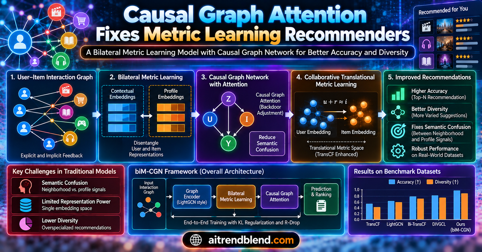
Key points
- biM-CGN combines bilateral translational metric learning with a causal graph network to fix a problem the authors call semantic confusion, where mixing neighborhood signals and profile signals in one embedding space quietly hurts performance.
- Simply combining LightGCN with TransCF, an apparently obvious upgrade, did not improve results in the authors’ own tests, which is what sent them looking for the underlying cause.
- The fix splits every user and item embedding into two spaces, one for contextual neighborhood information and one for the point representation itself.
- A structural causal model separates a causal factor that reflects genuine taste from a confounder that reflects noisy interaction, then blocks the confounder through backdoor adjustment.
- Two conditional intervention modules, one tied to the target item and one tied to user behavior, let the model trade off accuracy and diversity, and using both together gives the strongest result.
- On the Music dataset biM-CGN reaches a Recall at 5 of 0.1773 and an NDCG at 5 of 0.1796, ahead of LightGCN, DivGCL, EDUA star, and every other tested baseline.
An upgrade that should have worked and quietly did not
Recommender systems built on metric learning represent each user and item as a point in a shared space and push the distance between a user and the items they like to shrink relative to items they do not like. This sidesteps a known weakness of plain inner product similarity, which can violate the triangle inequality and produce inconsistent rankings. TransCF, introduced by Park and colleagues, improved on that basic idea by adding a translation vector between user and item, learned from the intensity and pattern of a user’s implicit interactions, which gives the model room to represent varied relationship types rather than forcing everything into one fixed distance.
Meanwhile graph neural networks, LightGCN chief among them, have repeatedly shown that folding in high order neighbor information, not just a user’s direct interactions but their neighbors’ neighbors, improves representation quality across recommendation tasks. Combining the two seems like free performance. The authors tried exactly that, updating TransCF’s node embeddings and translation vectors by aggregating high order neighbor signal the way LightGCN does, and building what they label LightGCN plus TransCF. Figure 2 in the paper shows the result on the Music and Beauty datasets, and it is not the win anyone expected. The combined model sits roughly on par with, and in some metrics behind, the two components run separately.
That negative result is the actual contribution people should pay attention to before jumping to the architecture. The paper spends real effort explaining why an intuitively sound combination fails, which is a more useful lesson for anyone building a similar system than the eventual fix.
Semantic confusion, the diagnosis behind the failure
The authors trace the problem to what they call semantic confusion. A user or item embedding in these models is being asked to carry two different kinds of information at once. One is contextual, meaning it comes from a node’s neighborhood, its interaction history, and the high order graph structure around it. The other is what the paper calls center or profile information, the point representation that anchors a user or item in the metric space itself. TransCF’s translation vectors were designed with the second kind of information in mind, encoding the intensity and heterogeneity of a user’s direct interactions. Feeding first the aggregated, neighborhood flavored embeddings from a GNN into that same machinery blurs the two signals together, and the model loses the clean distinction that made translation based metric learning work in the first place.
The proposed fix is direct. Split every user and item embedding into two separate vectors, one living in a contextual space and one in a profile space.
Here u^r and v^r carry the contextual, neighborhood derived signal, while u^c and v^c anchor the point in the profile space that the metric loss actually measures distance in. High order graph information still flows through both spaces, but the model no longer forces the two roles onto the same numbers.
The lineage of translation based metric learning, and where it gets shaky
Before landing on their fix, the authors walk through three earlier designs to show exactly where things break. Collaborative Metric Learning, the earliest of the three, maps users and items to single points and minimizes a triplet loss that pulls a positive item toward the user and pushes a negative item away by a margin. It works, but a single point per user or item cannot capture how the strength and character of a preference shifts depending on which item is being compared.
TransCF adds a translation vector on top of that point, computed with attention over the items a user has already interacted with, which lets the model express relationship intensity rather than a flat distance. Bi-TransCF decouples this into two channels, one predicting from user toward item and one from item toward user, so each side can optimize somewhat independently. Target aware Bi-TransCF goes further and lets the translation vector itself depend on which specific item or user is currently the target, rather than staying fixed.
Each step adds expressiveness, and each step also makes an old geometric guarantee harder to keep. Point based and translation based relationships are both supposed to respect the triangle inequality so that the model’s optimization has a clean path to follow. The paper shows, through the geometry in Figure 3, that once translation vectors are computed independently in the two directions, a paradox can appear where the model’s objective is satisfied looking one way but violated looking the other. That inconsistency becomes more visible once translation vectors are made target aware, since now the radius of influence for a positive item can legitimately exceed that of a negative item in one channel while the reverse holds in the other.
Looking at the recommendation score through a causal lens
Rather than patching the geometry further, the authors step back and ask what is actually determining a recommendation score. They build a structural causal model, shown in Figure 4 of the paper, treating the final score Y as a function of the user representation U, the user’s behavior representation E_X, and the target item representation E_t. The behavior representation itself splits along two causal paths. One path runs through X_p, a causal structure that captures which of a user’s past interactions genuinely relate to the current target, useful when someone has broad and varied interests and only some of their history is relevant right now. The other path runs through X_d, a confounder that reflects interactions which happened for reasons unrelated to real preference, noisy clicks, promotional exposure, or simple accident, and which the paper argues actively hurts satisfaction if left unaddressed.
Given the structure of the task, the authors show the prediction factorizes cleanly.
That factorization means the causal intervention work only needs to focus on the P(Y \mid V_t, X) term, since the path from X through the confounder X_d is the backdoor route that muddies the relationship between the causal factor and the outcome. To block it, the paper applies do calculus, intervening on X_p while holding the target fixed.
In plain terms, the model considers the outcome across the range of possible confounder values rather than letting whatever confounder happened to occur in the training data quietly bias the causal feature’s contribution. This is backdoor adjustment, a standard tool in causal inference, applied here to a recommendation scoring problem rather than the usual epidemiology or economics setting.
How the architecture puts this into practice
A disentangled graph network splits good signal from noise
For a given user and target item pair, the model needs to decide which of the user’s past interactions genuinely relate to that target. A gating mechanism handles this. Each historical item embedding in the contextual space is compared against the target item embedding through a learned gate.
The gate output, squeezed between zero and one by a sigmoid, marks which dimensions of a historical item’s embedding are actually relevant to the current target. That splits each historical item into a relevant factor and a residual factor.
A contrastive style loss then pushes the relevant factor closer to the target than the residual factor sits, so the gate actually learns to separate signal from noise rather than collapsing to a trivial split.
The residual factors from a user’s neighborhood are then combined through attention into the actual translation vector used downstream, with the attention weights computed by comparing each residual factor against the target in the contextual space while the user side of the calculation draws from the profile space, keeping the two roles apart the way the semantic confusion fix demands.
Both directions get their own translation, computed the same way
Because one way translation limits what the model can express, the framework computes both a user toward item translation and an item toward user translation, aggregating from each side’s own neighborhood using the same gated attention mechanism described above. That bilateral structure is where the M in biM-CGN comes from, bilateral metric learning paired with a causal graph network.
Conditional intervention generates the confounder on demand
Rather than trying to enumerate every possible confounder value, which would be impractical, the model generates a confounder specific condition directly from the target item and the user’s neighborhood.
Restricting the generation to the neighborhood, rather than the whole item catalog, keeps the process from introducing extra noise of its own. The authors also point out that diversity is worth optimizing directly, and that from a diversity standpoint the roles of causal factor and confounder can be swapped, which is where the second intervention module comes in, generated the same way but conditioned on user behavior instead of the target.
Both interventions get their own loss term, and the two combine into the full conditional intervention objective used during training.
Everything comes together in a pairwise margin loss that trains both translation directions at once, using the point embeddings from the profile space for the actual distance calculation while the translation vectors themselves come from the contextual space.
Datasets, baselines, and how the experiment was set up
The authors evaluate on three public datasets, two from Amazon review data (Digital Music and Beauty, using the 5-core filtered version that drops users and items with fewer than five interactions) and MovieLens using the 1M version. Ratings are converted to binary interaction signals for the top-N recommendation task.
| Dataset | Users | Items | Interactions | Sparsity | Categories |
|---|---|---|---|---|---|
| Music | 5541 | 3568 | 74786 | 99.67% | 60 |
| Beauty | 8159 | 5862 | 98566 | 99.79% | 41 |
| MovieLens-1M | 6040 | 3706 | 1000209 | 95.53% | 18 |
For each user, 80 percent of interactions form the training set and the remaining 20 percent form the test set, with every unobserved item ranked at test time. The model trains with the Adam optimizer, a batch size of 128, a maximum of 20 epochs, an initial learning rate of 0.0005, and an embedding dimension of 50. The margin used across every metric learning method, including biM-CGN, is fixed at 1.0 for a fair comparison, and biM-CGN samples 20 unobserved items per positive pair as negatives, matching the negative sampling used for LightGCN in the same experiments. Every reported number is averaged across five repeated runs.
Baselines span three families. Classical collaborative filtering includes LFM, NCF, and ENMF. Metric learning based methods include CML, TransCF, BGCF, and EDUA star, a version of EDUA with its adaptive balancing strategy removed so the comparison does not depend on item category metadata biM-CGN does not use. Graph based methods include LightGCN, DGRec, and DivGCL, the last of which the paper describes as the prior state of the art for balancing accuracy and diversity in GNN based recommendation.
How the results actually landed
On Music and MovieLens, biM-CGN clears every baseline by a clear margin. The paper reports a relative improvement over the strongest baseline of 3.4 percent on Recall at 5 and 4.3 percent on NDCG at 5 for Music, and 4.6 percent on Recall at 5 and 2.5 percent on NDCG at 5 for MovieLens.
| Method | Recall@5 | Recall@10 | NDCG@5 | NDCG@10 |
|---|---|---|---|---|
| CML | 0.1579 | 0.2204 | 0.1645 | 0.1879 |
| TransCF | 0.1598 | 0.2242 | 0.1611 | 0.1871 |
| EDUA star | 0.1544 | 0.2134 | 0.1615 | 0.1844 |
| LightGCN | 0.1633 | 0.2332 | 0.1663 | 0.1990 |
| DivGCL | 0.1633 | 0.2421 | 0.1663 | 0.2011 |
| biM-CGN (proposed) | 0.1773 | 0.2481 | 0.1796 | 0.2131 |
On the Beauty dataset, biM-CGN still posts the best Recall and NDCG figures in the table, though the authors are candid that the margin over ENMF feels smaller in practice than the headline numbers suggest, attributing ENMF’s strength to its whole data training strategy, which uses every unobserved interaction as a negative signal rather than sampling a subset. That is a more expensive training approach, and biM-CGN reaches comparable or better territory while sampling only 20 negatives per pair, a meaningfully cheaper setup.
The overall pattern across baselines is informative on its own. LFM and NCF, both leaning on matrix factorization style latent features, trail the rest of the field, suggesting that representation alone without an explicit distance metric or graph structure is not enough for these sparse datasets. LightGCN and BGCF post only modest gains over classical collaborative filtering, and the authors attribute part of that to BGCF trading precision for diversity by design, and part of it to LightGCN inheriting the very semantic confusion and triangle inequality issues this paper set out to fix. DGRec underperforms even the classical baselines, which the authors trace to its reweighting strategy toward long tail items leaving popular head items under trained, compounded by gradient vanishing under the datasets’ heavy sparsity.
What the ablation study reveals about each moving part
The authors test four stripped down variants against the full model. GCN_d removes the attention mechanism and replaces it with a plain graph convolution. Target_w/o removes target awareness. Disen_w/o removes the disentanglement gating. Confusion_w/o removes the embedding split between contextual and profile spaces entirely, effectively reintroducing the original semantic confusion problem.
| Variant (Music dataset) | Recall@5 | Recall@10 | NDCG@5 | NDCG@10 |
|---|---|---|---|---|
| GCN_d, attention removed | 0.1551 | 0.2081 | 0.1585 | 0.1795 |
| Confusion_w/o, embedding split removed | 0.1613 | 0.2299 | 0.1645 | 0.1905 |
| Disen_w/o, disentanglement removed | 0.1621 | 0.2211 | 0.1673 | 0.1935 |
| Target_w/o, target awareness removed | 0.1630 | 0.2311 | 0.1689 | 0.1966 |
| Layer-2, two graph attention layers | 0.1688 | 0.2391 | 0.1734 | 0.1991 |
Removing the embedding split hurts the most among these variants, which lines up directly with the paper’s core claim that solving semantic confusion is the single biggest lever in the whole design. Removing the disentanglement gating comes next, followed by removing target awareness. Interestingly, dropping the attention mechanism entirely and falling back to plain graph convolution only costs a modest amount of accuracy, especially on Beauty and MovieLens, which the authors credit to graph convolution’s built in Laplacian regularization already handling long tail effects reasonably well. Their practical suggestion is that GCN based metric learning is a workable, cheaper fallback when attention computation is too costly for a given deployment.
Layer depth follows the familiar graph neural network pattern. Two to three propagation layers give the best or second best results, since more hops let the model reflect higher order connectivity, but stacking beyond that starts to blur node representations together through over smoothing, matching what other GNN based recommendation work has already found.
Removing the embedding decoupling model performs worst, which means the decoupled embedding contributes the most to the whole model, followed by the disentanglement module. The paper’s own reading of its ablation results, Section 5.3.1
Trading off accuracy and diversity on purpose
A model that only chases Recall and NDCG can end up recommending the same handful of popular items to everyone, so the paper also measures intra list distance and category coverage as diversity metrics, combined with Recall into an F-score that rewards a genuine balance of the two. On Music, the fully combined model, using both the target conditioned and user conditioned intervention modules together, reaches an F1 at 10 of 0.3508, ahead of DivGCL at 0.3250 and EDUA at 0.3266. On Beauty the combined model reaches an F1 at 10 of 0.1937, again ahead of both of those diversity focused baselines. Compared with EDUA specifically, the paper reports a relative improvement of up to 7.4 percent on Music and 2.6 percent on Beauty at F1 at 10.
The two intervention variants behave differently on their own, and the paper is upfront about the tension. Conditioning on the target item alone tends to favor diversity at some cost to raw accuracy, while conditioning on user behavior alone tends to favor accuracy with less diversity gain, and the two together land in between while beating either alone on the combined metric. A separate visualization, using two randomly selected Music dataset users identified by ID 4682 and ID 2395, shows the attention distribution shifting depending on which item is the current target, and shows the disentanglement module assigning noticeably more weight to items that share the target’s category compared to a conventional GNN baseline, which is the kind of qualitative evidence that backs up the diversity numbers.
Honest limitations
The datasets here, while standard in the recommendation literature, are modest in scale next to production systems, topping out at roughly eight thousand users and six thousand items on Beauty and a little over a million interactions on MovieLens-1M. Sparsity above 99 percent on Music and Beauty means most user item pairs are unobserved by construction, and while that is realistic for e-commerce style data, it also means the evaluation protocol of ranking every unobserved item per user becomes computationally heavy at any larger scale, a cost the paper does not address.
The Beauty result also deserves a second look rather than a straight read of the bolded numbers. The authors themselves note that ENMF, a considerably simpler whole data training method, comes close to biM-CGN on that dataset, and while biM-CGN wins on paper, the practical gap a deployment team would notice is smaller there than on Music or MovieLens.
There is also a genuine tension in how the paper characterizes its own two intervention modules. One passage states that conditioning on the target favors diversity while conditioning on user behavior favors accuracy, and a later passage summarizing the same experiments states that user behavior conditioning improves both diversity and accuracy while target conditioning mainly adds robustness to noise. Both characterizations appear in the paper, and readers trying to reuse just one of the two intervention modules in isolation should look closely at Tables 4 and 5 rather than relying on the prose summary alone.
Finally, cold start users and items, a persistent headache for any interaction based recommender, do not get dedicated treatment here. The causal framing targets confounded historical interactions, not the absence of interaction history altogether, so it is unclear from the paper how biM-CGN would behave for a brand new user or a freshly listed item with no neighbors to draw on.
Where this fits in the bigger picture
The specific numbers matter less than the general lesson the negative result at the start of the paper teaches. Stacking a strong graph neural network on top of a strong metric learning head is not automatically additive, and anyone building a similar hybrid system would do well to check for the same kind of semantic confusion between neighborhood signal and point representation before assuming the combination will help. Causal disentanglement, splitting a signal into a genuinely predictive factor and a confounding factor and then applying backdoor adjustment, is also a pattern that keeps showing up across recommendation research dealing with popularity bias, selection bias, and now this semantic confusion problem, and it seems likely to keep spreading to other corners of the field where correlation quietly gets mistaken for user preference.
Conclusion
biM-CGN earns its place in the recommendation literature less because of any single new layer and more because of the diagnosis it offers. Bolting a graph neural network onto a translation based metric learning model, an upgrade that looks obviously beneficial on paper, quietly underperforms because the two components are fighting over what a user or item embedding is supposed to represent. Splitting that embedding into a contextual space and a profile space, then layering a structural causal model on top to separate genuine taste signal from confounding noise, recovers the expected gains and adds a real improvement in recommendation diversity along the way.
The conceptual shift worth carrying forward is treating a recommendation score as the output of a causal process rather than a purely correlational one. Backdoor adjustment through do calculus is a long established tool in causal inference, and its application here to block a confounder inside a graph based recommender is a specific, well motivated instance of a pattern that could transfer to other systems where noisy interaction data gets mistaken for genuine preference.
None of that erases the rough edges. The Beauty result sits closer to a strong simple baseline than the headline table suggests, the paper’s own prose gives two somewhat different accounts of what its two intervention modules actually specialize in, and cold start behavior is left unexamined. Those gaps mark out the next round of validation rather than undercut the core finding.
Where this heads next seems reasonably open. Testing the same contextual and profile space split against other GNN backbones beyond LightGCN, scaling the causal intervention modules to catalogs an order of magnitude larger, and directly reconciling the two competing explanations of what the target conditioned and user conditioned modules each contribute would all sharpen the picture considerably.
For anyone assembling a recommender that mixes graph propagation with a metric or translation based scoring head, the practical takeaway is straightforward, check whether the two components are quietly competing for the same representation before trusting that combining them will help, and consider whether a causal reframing of the confounder problem might do more for diversity than another round of architecture tuning.
Complete PyTorch implementation
The implementation below reconstructs the core pieces of biM-CGN, the dual space embedding split, the gated disentanglement module, bilateral attention based translation vectors, the conditional causal intervention module, all four loss terms, and a runnable smoke test on random dummy data.
# bim_cgn.py
# Reconstruction of the biM-CGN architecture described in
# "Enhancing collaborative translational metric learning with causal
# graph network", Neurocomputing 651 (2025) 130933.

import torch
import torch.nn as nn
import torch.nn.functional as F


class DualSpaceEmbedding(nn.Module):
    """Splits each user and item into a contextual space vector and
    a profile space vector, the fix for semantic confusion."""

    def __init__(self, num_entities, dim=50):
        super().__init__()
        self.contextual = nn.Embedding(num_entities, dim)
        self.profile = nn.Embedding(num_entities, dim)
        nn.init.normal_(self.contextual.weight, std=0.01)
        nn.init.normal_(self.profile.weight, std=0.01)

    def forward(self, ids):
        return self.contextual(ids), self.profile(ids)


class DisentangleGate(nn.Module):
    """Splits a neighbor's contextual embedding into a relevant
    factor and a residual factor with respect to a target item,
    Equations 6 through 8 in the paper."""

    def __init__(self, dim):
        super().__init__()
        self.w1 = nn.Linear(dim, dim, bias=False)
        self.w2 = nn.Linear(dim, dim, bias=False)

    def forward(self, neighbor_ctx, target_ctx):
        gate = torch.sigmoid(self.w1(neighbor_ctx) * self.w2(target_ctx))
        relevant = neighbor_ctx * gate
        residual = neighbor_ctx - relevant
        return relevant, residual


class BilateralTranslation(nn.Module):
    """Aggregates residual neighbor factors into a translation vector
    using softmax attention, computed in both the u to v and v to u
    directions, Equations 10 through 13."""

    def __init__(self, dim):
        super().__init__()
        self.gate = DisentangleGate(dim)

    def forward(self, neighbor_ctx, target_ctx):
        # neighbor_ctx: (batch, num_neighbors, dim)
        # target_ctx:   (batch, dim)
        target_expanded = target_ctx.unsqueeze(1).expand_as(neighbor_ctx)
        relevant, residual = self.gate(neighbor_ctx, target_expanded)

        scores = (residual * target_expanded).sum(dim=-1)
        attn = F.softmax(scores, dim=-1).unsqueeze(-1)
        translation = (attn * residual).sum(dim=1)
        return translation, relevant, residual


class ConditionalInterventionModule(nn.Module):
    """Generates a confounder specific condition from the target item
    and a neighborhood aggregate, Equation 14. Used twice, once
    conditioned on the target and once conditioned on user behavior."""

    def __init__(self, dim):
        super().__init__()
        self.w1 = nn.Linear(dim, dim, bias=False)
        self.w2 = nn.Linear(dim, dim, bias=False)

    def forward(self, neighborhood_agg, target_ctx):
        gate = torch.sigmoid(self.w1(neighborhood_agg) * self.w2(target_ctx))
        confounder_hat = torch.cat([target_ctx, target_ctx * gate], dim=-1)
        return confounder_hat


class BiMCGN(nn.Module):
    """Bilateral Metric learning with a Causal Graph Network.
    Combines the dual space embeddings, bilateral translation,
    and the two conditional intervention modules into one model."""

    def __init__(self, num_users, num_items, dim=50, num_layers=2):
        super().__init__()
        self.user_emb = DualSpaceEmbedding(num_users, dim)
        self.item_emb = DualSpaceEmbedding(num_items, dim)

        self.u2v_layers = nn.ModuleList(
            [BilateralTranslation(dim) for _ in range(num_layers)]
        )
        self.v2u_layers = nn.ModuleList(
            [BilateralTranslation(dim) for _ in range(num_layers)]
        )
        self.intervene_target = ConditionalInterventionModule(dim)
        self.intervene_user = ConditionalInterventionModule(dim)

    def forward(self, user_ids, target_item_ids, history_item_ids, history_user_ids):
        # history_item_ids: (batch, num_hist) items the user interacted with
        # history_user_ids: (batch, num_hist) users who interacted with the target item
        u_ctx, u_prof = self.user_emb(user_ids)
        v_ctx, v_prof = self.item_emb(target_item_ids)

        hist_v_ctx, _ = self.item_emb(history_item_ids)
        hist_u_ctx, _ = self.user_emb(history_user_ids)

        r_uv = v_ctx
        r_vu = u_ctx
        for layer in self.u2v_layers:
            r_uv, relevant_v, residual_v = layer(hist_v_ctx, v_ctx)
        for layer in self.v2u_layers:
            r_vu, relevant_u, residual_u = layer(hist_u_ctx, u_ctx)

        d_uv = ((u_prof + r_uv - v_prof) ** 2).sum(dim=-1)
        d_vu = ((v_prof + r_vu - u_prof) ** 2).sum(dim=-1)

        neighborhood_agg_u = hist_v_ctx.mean(dim=1)
        neighborhood_agg_v = hist_u_ctx.mean(dim=1)
        x_d_target = self.intervene_target(neighborhood_agg_u, v_ctx)
        x_d_user = self.intervene_user(neighborhood_agg_v, u_ctx)

        return {
            "d_uv": d_uv,
            "d_vu": d_vu,
            "relevant_v": relevant_v,
            "residual_v": residual_v,
            "relevant_u": relevant_u,
            "residual_u": residual_u,
            "x_d_target": x_d_target,
            "x_d_user": x_d_user,
            "v_ctx": v_ctx,
        }


def margin_distance(a, b, dim=-1):
    return ((a - b) ** 2).sum(dim=dim)


def disentangle_loss(target_ctx, residual, relevant, margin=1.0):
    """Equation 9. Pushes the relevant factor closer to the target
    than the residual factor sits."""
    d_residual = margin_distance(target_ctx, residual)
    d_relevant = margin_distance(target_ctx, relevant)
    return F.relu(d_residual - d_relevant + margin).mean()


def intervention_loss(target_ctx, residual, confounder_hat, margin=1.0):
    """Equation 15. Pushes the generated confounder condition to sit
    farther from the target than the residual factor does."""
    d_residual = margin_distance(target_ctx, residual)
    d_confounder = margin_distance(target_ctx, confounder_hat)
    return F.relu(d_residual - d_confounder + margin).mean()


def pairwise_margin_loss(d_pos, d_neg, margin=1.0):
    return F.relu(d_pos - d_neg + margin).mean()


def total_loss(model, batch, margin=1.0):
    """Equation 16, the combined pairwise margin loss plus the
    disentanglement and intervention terms in both directions."""
    pos_out = model(
        batch["user_ids"], batch["pos_item_ids"],
        batch["history_item_ids"], batch["history_user_ids"],
    )
    neg_out = model(
        batch["user_ids"], batch["neg_item_ids"],
        batch["history_item_ids"], batch["history_user_ids"],
    )

    rank_loss = pairwise_margin_loss(pos_out["d_uv"], neg_out["d_uv"], margin)
    rank_loss = rank_loss + pairwise_margin_loss(pos_out["d_vu"], neg_out["d_vu"], margin)

    l_dis = disentangle_loss(pos_out["v_ctx"], pos_out["residual_v"], pos_out["relevant_v"], margin)
    l_dis = l_dis + disentangle_loss(pos_out["v_ctx"], pos_out["residual_u"], pos_out["relevant_u"], margin)

    l_con = intervention_loss(pos_out["v_ctx"], pos_out["residual_v"], pos_out["x_d_target"], margin)
    l_con = l_con + intervention_loss(pos_out["v_ctx"], pos_out["residual_u"], pos_out["x_d_user"], margin)

    return rank_loss + l_dis + l_con


def train_one_epoch(model, loader, optimizer, margin, device):
    model.train()
    running_loss = 0.0
    for batch in loader:
        batch = {k: v.to(device) for k, v in batch.items()}
        optimizer.zero_grad()
        loss = total_loss(model, batch, margin)
        loss.backward()
        optimizer.step()
        running_loss += loss.item()
    return running_loss / len(loader)


@torch.no_grad()
def recall_at_k(distances, ground_truth_idx, k=5):
    """distances: (batch, num_candidates), lower means more relevant."""
    topk = distances.topk(k, largest=False).indices
    hits = (topk == ground_truth_idx.unsqueeze(1)).any(dim=1)
    return hits.float().mean().item()


if __name__ == "__main__":
    # Smoke test on random dummy data.
    device = torch.device("cuda" if torch.cuda.is_available() else "cpu")

    num_users, num_items, dim, num_hist = 200, 300, 50, 10
    model = BiMCGN(num_users, num_items, dim=dim, num_layers=2).to(device)
    optimizer = torch.optim.Adam(model.parameters(), lr=5e-4)

    batch = {
        "user_ids": torch.randint(0, num_users, (8,), device=device),
        "pos_item_ids": torch.randint(0, num_items, (8,), device=device),
        "neg_item_ids": torch.randint(0, num_items, (8,), device=device),
        "history_item_ids": torch.randint(0, num_items, (8, num_hist), device=device),
        "history_user_ids": torch.randint(0, num_users, (8, num_hist), device=device),
    }

    loss = total_loss(model, batch, margin=1.0)
    print("Combined loss on dummy batch", loss.item())

    out = model(batch["user_ids"], batch["pos_item_ids"],
                batch["history_item_ids"], batch["history_user_ids"])
    print("u to v distance shape", out["d_uv"].shape)

    dummy_scores = torch.rand(8, 50, device=device)
    dummy_truth = torch.randint(0, 50, (8,), device=device)
    print("Recall at 5 on random scores", recall_at_k(dummy_scores, dummy_truth, k=5))
Frequently asked questions
What does biM-CGN stand for
It stands for bilateral Metric learning combined with a Causal Graph Network, the name the authors give their full recommendation model.
Why does combining LightGCN with TransCF fail
The paper traces it to semantic confusion, where neighborhood derived signal from the graph network and the point representation used by the metric learning head end up mixed in the same embedding space, undoing the benefit each was supposed to bring.
What is the causal graph network actually doing
It builds a structural causal model that separates a causal factor genuinely tied to user preference from a confounder that reflects noisy or incidental interactions, then applies backdoor adjustment to block the confounder’s influence on the recommendation score.
Does biM-CGN improve diversity or just accuracy
Both. The paper reports gains in Recall and NDCG alongside gains in intra list distance and category coverage, combined into an F-score that reached 0.3508 at 10 on the Music dataset, ahead of the diversity focused baselines DivGCL and EDUA.
What datasets was it tested on
Two Amazon review datasets, Digital Music and Beauty, both using the 5-core filtered version, plus the MovieLens-1M dataset.
Is this ready to use in a production recommender
The paper presents research results on three public benchmark datasets, each modest by production standards, with a compute heavy evaluation protocol that ranks every unobserved item per user. The authors do not address how the causal intervention modules would scale to a much larger catalog or handle cold start users and items.
Read the full study and explore the underlying datasets.
Read the paper on ScienceDirect Get the MovieLens dataset
Wang, J., Xie, H., Qin, S. J., Tao, X., Wang, F. L. and Xu, X. Enhancing collaborative translational metric learning with causal graph network. Neurocomputing 651, 130933 (2025). https://doi.org/10.1016/j.neucom.2025.130933. Supported by the Primary R&D Plan of Zhejiang, grant 2023C03198, Lingnan University Faculty Research Grants DB24A4 and SDS24A8 and Direct Grant DR25E8, the 2023 Nanjing International Hong Kong Macao and Taiwan Science and Technology Cooperation Program grant 202308010, and Research Grants Council of Hong Kong grants R1015 23 and UGC FDS16 E17 23. Published under a Creative Commons Attribution NonCommercial license.
This analysis is based on the published paper and an independent evaluation of its claims.