
- Quantum machine learning
- Molecular activity prediction
- Multimodal fusion
- Amplitude encoding
- Variational circuits
- Drug discovery
- PyTorch
A medicinal chemistry team has a list of a few thousand candidate compounds and a budget to synthesise perhaps fifty. Before anyone touches a flask, a model ranks the list by how likely each molecule is to bind a kinase or cross the blood brain barrier. A better ranking means fewer wasted syntheses, which is why molecular activity prediction has become one of the busiest corners of applied machine learning.
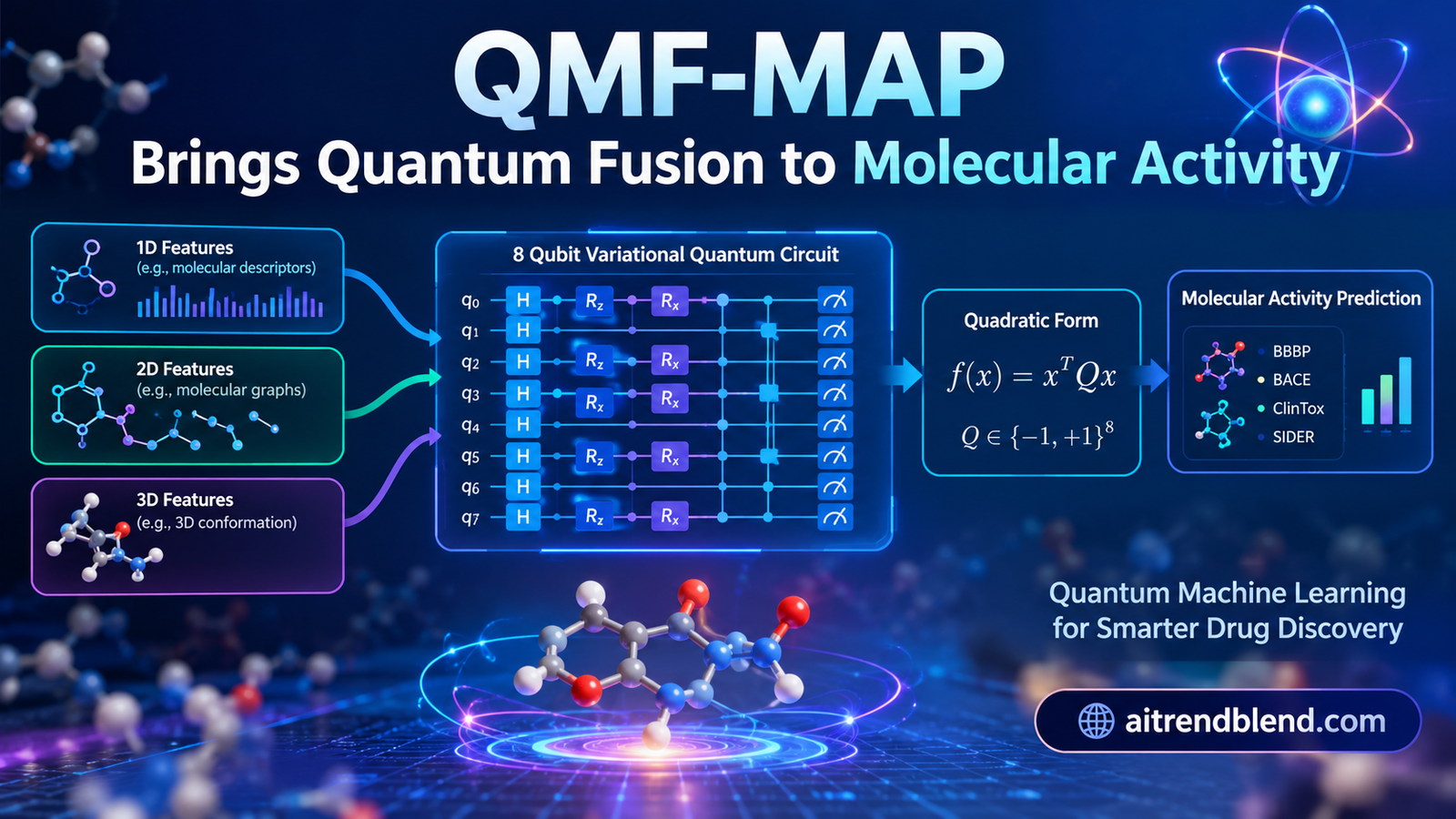
Maoduo Li, Wen Liu and colleagues at the Communication University of China, Changsha University of Science and Technology and Anhui University of Science and Technology bring quantum computing to that ranking problem. Their model, QMF-MAP, combines a molecule’s fingerprint, its 2D bond graph and its 3D shape, loads the result into eight qubits and lets a trainable quantum circuit decide. On eight benchmarks it matches or beats strong classical models. We reconstructed the circuit, and found that what it computes can be written down in one line of classical algebra.
Key points
- QMF-MAP extracts fingerprint, 2D graph and 3D bond angle features classically, projects their 632 dimensional concatenation to 256 numbers and amplitude encodes them into eight qubits for a quantum attention module and a pooled variational circuit.
- Its best reported results include an AUC of 0.940 on THR and 0.918 on BBBP, and it beats a classical attention plus MLP head on four datasets, by up to 11 AUC points on ClinTox.
- We prove and confirm numerically that the entire quantum part computes a quadratic form of the normalised input vector, with a 256 by 256 matrix whose eigenvalues are plus and minus one.
- As described in the paper, the quantum attention scores come from qubits prepared in a fixed state, so they are identical for every molecule. Our reconstruction confirms this.
- The reported classical parameter count of 6,324 cannot include the 632 to 256 projection, which alone needs 162,048 parameters.
- The BBBP F1 of 0.911 is impossible given the reported precision of 0.810 and recall of 0.848. All results come from a single random split, and ClinTox’s test set holds only about 11 active molecules.
Why activity prediction is a multimodal problem
A molecule can be described in at least three ways. As a string, such as a SMILES code, which can be turned into a fingerprint of substructures. As a graph of atoms and bonds, which captures connectivity. And as a 3D shape, where bond angles and distances decide how the molecule fits into a protein pocket. Two molecules with the same graph can have different shapes and different activities, so each view carries something the others miss.
Classical models have exploited each view in turn. D-MPNN, from Yang and colleagues, refines message passing on bonds. AttentiveFP, from Xiong and colleagues, adds graph attention. Uni-Mol learns from 3D conformations, and pretrained models such as GROVER, MolCLR and Mole-BERT learn from millions of unlabelled molecules. Multimodal models that combine views, such as the dynamic weighting approach of Yi and colleagues, generally beat single view ones.
The QMF-MAP authors argue that classical fusion struggles with feature coupling and alignment in high dimensional molecular spaces, and that quantum circuits, which can hold \(2^n\) numbers in \(n\) qubits, offer a resource efficient alternative. Quantum models have already been tried for multimodal sentiment analysis and fake news detection. This is, as far as the authors know, the first application to molecular activity.
How QMF-MAP is built
Three classical feature extractors
For the 1D view, an Extended Connectivity Fingerprint is computed from the SMILES string and embedded with Mol2vec, a word2vec style model for substructures. For the 2D view, atoms are embedded with a continuous bag of words model over their neighbourhoods, then combined along walks of increasing length in an N gram graph scheme. For the 3D view, RDKit generates and energy minimises a conformation, a bond angle graph is built with bonds as nodes and angles as edges, and a GeoGNN style network produces a vector. The three vectors are concatenated into one of length 632.
The fully connected layer \(F\) maps 632 numbers to \(2^n\), with \(n = 8\) qubits and so 256 numbers in the main configuration. It is trained jointly with the circuit.
Amplitude encoding
The 256 numbers are normalised and become the amplitudes of an 8 qubit state.
Quantum attention
A set of auxiliary qubits, initialised in the equal superposition state, passes through a shallow trainable circuit \(V\). Measuring observables \(O_{ij}\) gives raw scores, a softmax gives weights, and the weights scale the angles of controlled \(R_y\) rotations between data qubits.
A pooled variational circuit
The attended state then passes through three variational layers, each with \(R_x\) and \(R_y\) rotations around a ring of CNOT gates, interleaved with two qubit pooling units that entangle a pair and discard one qubit, in the style of the quantum convolutional networks of Cong and colleagues. Eight qubits shrink to four, then two, then one. The prediction is read from a Pauli Z measurement on the last qubit.
Training uses focal loss with a class weight tuned per dataset, and the parameter shift rule for gradients. Everything quantum is simulated in PennyLane on a classical machine.
What the eight qubit circuit actually computes
Here is where it gets interesting. Take any circuit of this kind, with amplitude encoding at the start, any sequence of unitary gates in the middle and a single Pauli measurement at the end. Pooling looks different because it discards qubits, but a discarded qubit that is never measured or touched again is the same as one that is simply ignored. So the whole quantum part, attention included, is one fixed 256 by 256 unitary \(U\) followed by measuring \(Z\) on one qubit. In the Heisenberg picture, that is a single observable.
Because the encoded amplitudes are real, only the real part of the observable matters. And because \(Z \otimes I\) has 128 eigenvalues of plus one and 128 of minus one, so does \(U^{\dagger}(Z\otimes I)U\). The quantum model is therefore a classical normalised quadratic form, with a symmetric matrix drawn from a specific family and parameterised by about 170 rotation angles.
We checked this directly. We built the attention module, three variational layers and pooling in an exact state vector simulator, extracted \(U\) by running every basis state through it, and compared the circuit’s output with \(\hat x’^{\top} S \hat x’\) on random inputs. The largest difference was 1.2 times 10 to the minus 7, which is floating point rounding. The observable had exactly 128 eigenvalues at plus one and 128 at minus one.
Eight qubits hold 256 numbers. A circuit that reads them out with one measurement is a 256 by 256 matrix in disguise. aitrendblend analysis of QMF-MAP, Information Fusion 2027
This is not a criticism of quantum machine learning in general. It is a statement about scale. At eight qubits, everything the circuit does can be computed exactly on a laptop with one matrix multiplication per molecule, so any claim of exponential representation buys nothing here. Two consequences follow. A model with real quantum advantage would need many more qubits, or data that is itself quantum, or measurements whose statistics are hard to simulate. And a fair classical comparison for QMF-MAP is not an attention block plus a three layer MLP, but the same projection followed by a learned quadratic form. In our synthetic test, that classical quadratic head reached a test AUC of 0.984 where the simulated circuit reached 0.957.
For amplitude encoded variational classifiers on a handful of qubits, the circuit is a constrained quadratic model of the normalised input. Any reported quantum gain should be compared against that classical model, which costs one matrix product to evaluate.
The attention does not look at the molecule
The paper describes the attention module’s auxiliary qubits as starting from a fixed superposition state, passing through a trainable circuit and being measured. Nothing in that description loads the molecule’s features into those qubits. If that is how the model works, the scores \(\beta_{ij}\), and so the weights \(\alpha_{ij}\), are the same for every input. They are learned constants, and the module reduces to a layer of controlled rotations with angles \(\theta_{ij}\alpha_{ij}\), a reparameterisation of trainable angles.
Our reconstruction confirms the consequence. For two random molecules, the attention weights were identical. That matters for the paper’s interpretation, which reads the ablation as showing that quantum attention dynamically emphasises 3D features for structurally complex molecules and 2D topology for others. With input independent weights, the module cannot adapt per molecule. It could only differ between datasets, because a separate model is trained for each one. The ablation’s 3.6 point average AUC gain from adding the module is consistent with simply adding another trainable layer.
It is possible that the implementation differs from the text, for example by loading features into the auxiliary register. No code was released with the paper, so we cannot check.
What the experiments show
The evaluation uses eight binary datasets. Four come from ChEMBL, ABL kinase, caspase protease, thyroid hormone receptor and hepatocyte growth factor receptor, labelled by IC50 thresholds. Four come from MoleculeNet, BACE, ClinTox, BBBP and the first SIDER subtask. All are split at random 8 to 1 to 1 with seed 42, and all baselines were retrained on the same split.
| Dataset | Molecules | Active | Accuracy | Precision | Recall | F1 | ROC AUC |
|---|---|---|---|---|---|---|---|
| ABL | 2,644 | 2,127 | 0.772 | 0.706 | 0.807 | 0.719 | 0.861 |
| CASPASE | 709 | 315 | 0.850 | 0.848 | 0.849 | 0.848 | 0.913 |
| THR | 654 | 338 | 0.876 | 0.877 | 0.876 | 0.876 | 0.940 |
| HGFR | 4,440 | 3,941 | 0.873 | 0.831 | 0.829 | 0.752 | 0.884 |
| BACE | 1,513 | 691 | 0.774 | 0.782 | 0.781 | 0.774 | 0.880 |
| ClinTox | 1,484 | 112 | 0.845 | 0.630 | 0.791 | 0.660 | 0.877 |
| BBBP | 2,039 | 1,560 | 0.843 | 0.810 | 0.848 | 0.911 | 0.918 |
| SIDER HD | 1,427 | 743 | 0.713 | 0.701 | 0.701 | 0.699 | 0.738 |
Table A. QMF-MAP results from Tables 1 and 2 of Li et al. Precision, recall and F1 are macro averages. The highlighted BBBP F1 is discussed below.
Against nine classical models on the four MoleculeNet datasets, QMF-MAP has the best AUC on SIDER, 0.738, and BACE, 0.884 against GROVER’s 0.882. It is third on BBBP, at 0.918 behind Mole-BERT at 0.929 and Uni-Mol at 0.926, and second on ClinTox, 0.884 against Uni-Mol’s 0.885. The abstract’s claim of superior or comparable performance is fair, though comparable describes most of the table better than superior.
The modality ablation is clean and useful. Averaged over the eight datasets, accuracy was 0.737 with fingerprints only, 0.784 with 2D graphs only and 0.775 with 3D only. The best pair, 2D plus 3D, reached 0.814, and all three together 0.817. Almost all of the multimodal gain comes from combining topology and geometry, and fingerprints add very little on top. That is a practical finding regardless of what sits downstream.
Quantum versus classical heads
| Dataset | Head | Accuracy | F1 | ROC AUC |
|---|---|---|---|---|
| BBBP | Attention plus 3 layer MLP | 0.813 | 0.816 | 0.880 |
| QMF-MAP | 0.843 | 0.828 | 0.918 | |
| BACE | Attention plus 3 layer MLP | 0.751 | 0.756 | 0.862 |
| QMF-MAP | 0.774 | 0.774 | 0.880 | |
| SIDER HD | Attention plus 3 layer MLP | 0.632 | 0.663 | 0.666 |
| QMF-MAP | 0.713 | 0.699 | 0.738 | |
| ClinTox | Attention plus 3 layer MLP | 0.769 | 0.616 | 0.791 |
| QMF-MAP | 0.845 | 0.660 | 0.877 |
Table B. Classical multimodal baseline against QMF-MAP on identical input features, from Table 6 of Li et al.
Including this comparison was the right instinct, and the gains look consistent. Two cautions apply. The classical head is a different model class rather than the classical equivalent of the circuit, and its tuning is not described. And the largest gains are on the smallest test sets, where noise is largest, as we show next.
Noise and resources
With noise channels applied after every gate during training, BACE AUC fell from 0.880 to between 0.861 and 0.877 at an error rate of 0.01, and to between 0.801 and 0.858 at 0.1, with depolarising noise the most damaging. The circuit uses 30N minus 6 gates and 21N parameters, 234 gates and 168 parameters at eight qubits. On a CPU simulator, training took 16 seconds per epoch on BBBP, against under 1 second for five of the eight classical baselines on a GPU, with GROVER at 19.8 seconds and D-MPNN at 80 seconds the slow exceptions.
Checking the numbers
An impossible F1. For macro averages, each class’s F1 is a harmonic mean, which never exceeds the arithmetic mean of that class’s precision and recall. Averaging over classes, macro F1 can be no larger than the average of macro precision and macro recall. For BBBP, that ceiling is \((0.810 + 0.848)/2 = 0.829\). The reported 0.911, in both Table 2 and Table 3, cannot be right. Table 6 reports 0.828 for the same model and dataset, which fits the bound and is likely the correct value. The 0.911 in Table 3 is also what makes QMF-MAP look competitive on BBBP F1.
Values that differ between tables. ClinTox AUC is 0.877 in Tables 2 and 6 but 0.884 in Table 3 and the text. BACE AUC is 0.880 in Tables 2, 6 and 8 but 0.884 in Table 3. BBBP multimodal accuracy is 0.843 in Table 2 and 0.833 in Table 4.
Parameter count. Table 10 lists QMF-MAP with 6,324 classical and 168 quantum parameters, against about 18 thousand to 3.6 million for the classical baselines. A fully connected layer from 632 inputs to 256 outputs has \(632 \times 256 + 256 = 162{,}048\) parameters, 25 times the reported classical count. The Mol2vec, N gram and GeoGNN extractors are not counted at all. The model is far larger than 6,500 parameters. Whether it is smaller than the baselines depends on how those extractors are counted.
Split and sample size. The setup says every dataset was split at random with seed 42, yet the results section twice describes scaffold split generalisation benchmarks. Random splits put close analogues of test molecules in the training set and generally give higher scores than scaffold splits, which is why scaffold splits are standard for MoleculeNet. And with one split and no repeated runs, there is no estimate of variance. We estimated the test set composition from the dataset statistics and the 8 to 1 to 1 split.
| Dataset | Approx. test molecules | Approx. active | Approx. inactive | Reported AUC | Rough 95 percent range |
|---|---|---|---|---|---|
| ClinTox | 148 | 11 | 137 | 0.877 | 0.74 to 1.0 |
| THR | 65 | 34 | 31 | 0.940 | 0.88 to 1.0 |
| CASPASE | 71 | 32 | 39 | 0.913 | 0.84 to 0.99 |
| SIDER HD | 143 | 74 | 69 | 0.738 | 0.66 to 0.82 |
| BACE | 151 | 69 | 82 | 0.880 | 0.82 to 0.94 |
Table C. Our approximate test set sizes and Hanley and McNeil style intervals, assuming class proportions are preserved by the random split. Treat these as orders of magnitude, not exact intervals.
With about 11 active compounds in the ClinTox test set, an AUC of 0.877 is compatible with anything from about 0.74 to 1.0. The classical baseline’s 0.791 sits inside that range, so the headline 11 point ClinTox gain could be noise. THR and CASPASE, with about 65 and 71 test molecules, are also small.
The zero padding ablation. To test the projection layer, the authors compared learned projections to 256, 512 and 1024 dimensions with zero padding the 632 features to 1024. Zero padding performed very badly, with accuracy 0.456, macro recall exactly 0.500 and AUC 0.642, and the paper concludes that padding without a learnable transform is insufficient. But amplitude encoding normalises the vector, and padding with zeros changes nothing except adding empty amplitudes. No information is lost. A macro recall of exactly 0.5 means the model predicted a single class for every molecule. This looks like a training failure, perhaps from unscaled raw features, rather than evidence that the projection preserves information. The same table shows 10 qubits giving a better AUC, 0.904, than the 8 qubits adopted, 0.880.
Expressibility and trainability. The circuit’s expressibility, a KL divergence of 0.0002 from the Haar random distribution, is presented as both a strength and as potentially mitigating barren plateaus. In the quantum machine learning literature, circuits whose outputs look Haar random are usually the ones that suffer barren plateaus, with gradients that shrink exponentially in the number of qubits. At eight qubits this is manageable, so it is not a problem for the experiments, but it is the opposite of reassurance for the scaled up hardware version the paper envisions.
What running this on quantum hardware would take
The paper argues that the 16 seconds per epoch is a simulation artefact and that native hardware would be more efficient, since circuit depth grows only logarithmically with feature dimension. Three costs are missing from that argument. Preparing an arbitrary amplitude encoded state of 256 numbers generally needs a number of gates that grows with the vector length, not its logarithm, and the gate count of 234 excludes it. Each prediction is a probability estimated from repeated measurements, so every molecule needs many shots. And the parameter shift rule needs two circuit evaluations per parameter per gradient, so one gradient step on one molecule means 336 circuits, each with its own shots. For this model size, a classical computer evaluates the equivalent quadratic form faster than any current device could prepare the state.
None of this rules out quantum models for chemistry. Molecules are quantum systems, and hybrid models that work with quantum mechanical descriptions directly, or with many more qubits, may eventually earn an advantage. Physics aware classical models already go that way, as our piece on force free molecular dynamics with equivariant networks shows. But for classical feature vectors on a few qubits, as here, the honest framing is a compact constrained classifier, not a quantum speedup.
Where QMF-MAP fits
The useful findings in this paper do not depend on the quantum part. The modality ablation shows that combining 2D topology with 3D bond angle geometry gives most of the multimodal benefit, which is worth knowing for anyone building activity predictors. The noise study is a reasonable template for reporting robustness of variational circuits. And including a classical head with identical inputs is a practice more quantum machine learning papers should adopt.
For readers following quantum machine learning on this site, QMF-MAP fits a pattern we have seen before. Quantum-Gated LiteSSD for sonar detection also uses small circuits as one component in a larger classical network, and our review of robot path planning from search to quantum finds a similar gap between quantum promise and what small devices deliver today. For drug discovery more broadly, XPert, which predicts how drugs change cells, shows another way learned models enter the screening pipeline. On the evaluation side, our analysis of classification metrics explains the macro averaging bounds we used to check the F1 values above.
Limitations
Model description. As described, the quantum attention scores are input independent, and the paper’s interpretation of per molecule modality weighting cannot follow from them. No code was released to check the implementation.
Classical equivalence. At eight qubits the circuit is a quadratic form of the normalised input. The paper does not compare against this equivalent classical model, only against a different classical head.
Reporting errors. The BBBP F1 of 0.911 violates a mathematical bound. AUC and accuracy values differ between tables. The classical parameter count omits the projection layer and the feature extractors. The text describes scaffold splits that the setup says were not used.
Statistics. One random split with one seed, no repeated runs, no confidence intervals and very small test sets for ClinTox, THR and CASPASE. Several reported gains are within plausible noise.
Scope. All quantum computation is simulated. The noise study uses one dataset. Results are binary classification only, with SIDER reduced to a single subtask.
Reproducing QMF-MAP in PyTorch
The listing below is our independent reconstruction in plain PyTorch, with an exact batched state vector simulator in place of PennyLane. It implements amplitude encoding, the quantum attention module as described, with auxiliary qubits in a fixed superposition, a hardware efficient circuit, \(Z_iZ_j\) scores, a softmax and controlled \(R_y\) gates, three variational layers with cyclic CNOT rings, two qubit pooling from eight qubits down to one, the Z readout, focal loss, a training loop and AUC. It then runs the checks reported above, input independent attention, exact equality with the quadratic form and the plus and minus one spectrum, and trains both the circuit and a classical quadratic head on a synthetic 632 feature task.
Our circuit has 180 quantum parameters against the paper’s 168, because the exact attention parameterisation is not fully specified. The projection layer has 162,048 parameters, as computed above. Gradients flow through the simulator with automatic differentiation, which gives the same values the parameter shift rule would.
# QMF-MAP reconstruction and classical equivalence check (aitrendblend)
# Based on Li, Liu, Shi, Li, Chen and Zhang, "QMF-MAP, a quantum multimodal fusion model for
# molecular activity prediction", Information Fusion 137 (2027) 104584.
# Independent reconstruction in plain PyTorch with an exact state vector simulator.
# No official code was released with the paper, so circuit details follow the text and figures.
#
# Contents
#   1. a small batched state vector simulator (Rx, Ry, Rz, CNOT, controlled Ry)
#   2. amplitude encoding, the quantum attention module, VQC layers and 2 qubit pooling
#   3. the hybrid model, classical projection 632 -> 256 plus an 8 qubit circuit
#   4. checks, attention scores do not depend on the input as described, and the whole
#      circuit equals a quadratic form x^T S x of the normalised encoded vector
#   5. focal loss, training loop, AUC and a smoke test against a classical quadratic head

import math
import torch
import torch.nn as nn
import torch.nn.functional as F

CDT = torch.complex64

# ---------------------------------------------------------------------------
# 1. State vector simulator, state has shape (batch, 2, 2, ..., 2)
# ---------------------------------------------------------------------------
def rx(t):
    c, s = torch.cos(t / 2), torch.sin(t / 2)
    return torch.stack([torch.stack([c + 0j, -1j * s]), torch.stack([-1j * s, c + 0j])]).to(CDT)


def ry(t):
    c, s = torch.cos(t / 2), torch.sin(t / 2)
    return torch.stack([torch.stack([c, -s]), torch.stack([s, c])]).to(CDT)


def rz(t):
    e = torch.exp(-0.5j * t.to(CDT))
    return torch.stack([torch.stack([e, torch.zeros_like(e)]), torch.stack([torch.zeros_like(e), e.conj()])])


def apply_1q(state, gate, q):
    """Apply a 2x2 gate on qubit q. state (B, 2, ..., 2)."""
    s = torch.movedim(state, q + 1, -1)
    s = s @ gate.T
    return torch.movedim(s, -1, q + 1)


def apply_controlled(state, gate, ctrl, tgt):
    """Apply gate on tgt when ctrl is 1."""
    s = torch.movedim(state, (ctrl + 1, tgt + 1), (-2, -1))
    s0, s1 = s[..., 0, :], s[..., 1, :] @ gate.T
    s = torch.stack([s0, s1], dim=-2)
    return torch.movedim(s, (-2, -1), (ctrl + 1, tgt + 1))


X = torch.tensor([[0, 1], [1, 0]], dtype=CDT)


def cnot(state, c, t):
    return apply_controlled(state, X, c, t)


def expect_z(state, q):
    p = state.abs() ** 2
    p = torch.movedim(p, q + 1, -1)
    return (p[..., 0] - p[..., 1]).flatten(1).sum(1)


# ---------------------------------------------------------------------------
# 2. Encoding, attention, VQC and pooling (Eqs. 11 to 23)
# ---------------------------------------------------------------------------
def amplitude_encode(x, n):
    """Eq. 11, x of length 2^n is normalised and becomes the amplitudes."""
    x = F.normalize(x, dim=1).to(CDT)
    return x.reshape(x.shape[0], *([2] * n))


class QuantumAttention(nn.Module):
    """Eqs. 12 to 17. Auxiliary qubits start in |+> as the paper states, a hardware efficient
    VQC V acts on them, Z_i Z_j expectations give raw scores beta_ij, a softmax over j gives
    alpha_ij, and controlled Ry(theta_ij * alpha_ij) gates act on the data qubits."""
    def __init__(self, n):
        super().__init__()
        self.n = n
        self.v = nn.Parameter(torch.randn(2, n, 2) * 0.5)        # two layers of Rx, Ry on aux
        self.theta = nn.Parameter(torch.randn(n, n) * 0.5)        # original CRy angles

    def scores(self):
        n = self.n
        aux = torch.ones(1, *([2] * n), dtype=CDT) / math.sqrt(2 ** n)   # |+>^n
        for layer in range(2):
            for q in range(n):
                aux = apply_1q(aux, rx(self.v[layer, q, 0]), q)
                aux = apply_1q(aux, ry(self.v[layer, q, 1]), q)
            for q in range(n):
                aux = cnot(aux, q, (q + 1) % n)
        p = (aux.abs() ** 2)[0]
        beta = torch.zeros(n, n)
        for i in range(n):
            for j in range(n):
                zi = torch.movedim(p, i, 0); zi = zi[0] - zi[1]
                if i == j:
                    beta[i, j] = zi.sum()
                else:
                    jj = j if j < i else j - 1
                    zij = torch.movedim(zi, jj, 0)
                    beta[i, j] = (zij[0] - zij[1]).sum()
        return torch.softmax(beta, dim=1)                          # Eq. 14

    def forward(self, state):
        alpha = self.scores()
        for i in range(self.n):
            for j in range(self.n):
                if i != j:
                    state = apply_controlled(state, ry(self.theta[i, j] * alpha[i, j]), i, j)
        return state, alpha


class VQCLayer(nn.Module):
    """Eqs. 18 to 20, Rx Ry rotations, a cyclic CNOT ring, Rx Ry rotations, on chosen qubits."""
    def __init__(self, qubits):
        super().__init__()
        self.q = qubits
        self.t = nn.Parameter(torch.randn(2, len(qubits), 2) * 0.5)

    def forward(self, state):
        for k in range(2):
            for idx, q in enumerate(self.q):
                state = apply_1q(state, rx(self.t[k, idx, 0]), q)
                state = apply_1q(state, ry(self.t[k, idx, 1]), q)
            if k == 0:
                for idx in range(len(self.q)):
                    state = cnot(state, self.q[idx], self.q[(idx + 1) % len(self.q)])
        return state


class Pool(nn.Module):
    """Eq. 21, Rx Ry on q0, CNOT(q0, q1), Ry Rz on q1. q0 is then ignored (Eq. 22)."""
    def __init__(self):
        super().__init__()
        self.t = nn.Parameter(torch.randn(4) * 0.5)

    def forward(self, state, q0, q1):
        state = apply_1q(state, rx(self.t[0]), q0)
        state = apply_1q(state, ry(self.t[1]), q0)
        state = cnot(state, q0, q1)
        state = apply_1q(state, ry(self.t[2]), q1)
        return apply_1q(state, rz(self.t[3]), q1)


class QNN(nn.Module):
    """Three VQC stages with pooling, 8 -> 4 -> 2 -> 1 active qubits (Eq. 23)."""
    def __init__(self, n=8):
        super().__init__()
        assert n == 8
        self.stages = [[0, 1, 2, 3, 4, 5, 6, 7], [1, 3, 5, 7], [3, 7]]
        self.vqc = nn.ModuleList([VQCLayer(s) for s in self.stages])
        self.pools = nn.ModuleList([Pool() for s in self.stages for _ in range(len(s) // 2)])
        self.out_qubit = 7

    def forward(self, state):
        k = 0
        for s, vqc in zip(self.stages, self.vqc):
            state = vqc(state)
            for a, b in zip(s[0::2], s[1::2]):
                state = self.pools[k](state, a, b); k += 1
        return state


class QMFMAP(nn.Module):
    """Classical projection F (632 -> 2^n), amplitude encoding, quantum attention, QNN, <Z>."""
    def __init__(self, d_in=632, n=8, attention=True):
        super().__init__()
        self.n = n
        self.proj = nn.Linear(d_in, 2 ** n)                        # Eq. 10
        self.att = QuantumAttention(n) if attention else None
        self.qnn = QNN(n)

    def circuit(self, xq):
        state = amplitude_encode(xq, self.n)
        if self.att is not None:
            state, _ = self.att(state)
        state = self.qnn(state)
        return expect_z(state, self.qnn.out_qubit)

    def forward(self, x):
        z = self.circuit(self.proj(x))
        return (1 - z) / 2                                         # Eq. 26, probability of active


# ---------------------------------------------------------------------------
# 3. The classical equivalent of the circuit
# ---------------------------------------------------------------------------
@torch.no_grad()
def circuit_observable(model):
    """Build O = U^dagger Z_out U by running the circuit on every basis state, then return
    S = Re(O). For real amplitude encoded inputs, <Z> = x_hat^T S x_hat exactly."""
    n = model.n
    eye = torch.eye(2 ** n)
    state = eye.to(CDT).reshape(2 ** n, *([2] * n))
    if model.att is not None:
        state, _ = model.att(state)
    state = model.qnn(state)
    U = state.reshape(2 ** n, 2 ** n).T                            # column k is U|k>
    zdiag = torch.tensor([1.0 if ((k >> (n - 1 - model.qnn.out_qubit)) & 1) == 0 else -1.0
                          for k in range(2 ** n)], dtype=CDT)
    O = U.conj().T @ (zdiag[:, None] * U)
    return O.real, torch.linalg.eigvalsh(O)


class QuadraticHead(nn.Module):
    """Classical stand in, same projection, then p = (1 - x_hat^T S x_hat) / 2 with S learned."""
    def __init__(self, d_in=632, d=256):
        super().__init__()
        self.proj = nn.Linear(d_in, d)
        self.A = nn.Parameter(torch.randn(d, d) * 0.01)

    def forward(self, x):
        xh = F.normalize(self.proj(x), dim=1)
        S = (self.A + self.A.T) / 2
        return (1 - torch.tanh((xh @ S * xh).sum(1))) / 2


# ---------------------------------------------------------------------------
# 4. Focal loss, training and AUC
# ---------------------------------------------------------------------------
def focal_loss(p, y, alpha=0.5, gamma=2.0, eps=1e-6):
    p = p.clamp(eps, 1 - eps)
    return (-alpha * y * (1 - p) ** gamma * torch.log(p)
            - (1 - alpha) * (1 - y) * p ** gamma * torch.log(1 - p)).mean()


def auc(score, y):
    order = torch.argsort(score)
    r = torch.empty_like(score); r[order] = torch.arange(1, len(score) + 1, dtype=score.dtype)
    pos = y == 1; n1, n0 = pos.sum().item(), (~pos).sum().item()
    return ((r[pos].sum() - n1 * (n1 + 1) / 2) / (n1 * n0)).item()


def train(model, x, y, epochs=25, lr=1e-2, bs=32):
    """Autograd through the exact simulator. On hardware this would be the parameter shift rule."""
    opt = torch.optim.Adam(model.parameters(), lr=lr)
    sched = torch.optim.lr_scheduler.CosineAnnealingLR(opt, epochs)
    for _ in range(epochs):
        perm = torch.randperm(len(y))
        for i in range(0, len(y), bs):
            b = perm[i:i + bs]
            loss = focal_loss(model(x[b]), y[b])
            opt.zero_grad(); loss.backward(); opt.step()
        sched.step()
    return model


# ---------------------------------------------------------------------------
# 5. Smoke test
# ---------------------------------------------------------------------------
if __name__ == "__main__":
    torch.manual_seed(0)
    model = QMFMAP()
    n_q = sum(p.numel() for n_, p in model.named_parameters() if not n_.startswith("proj"))
    n_c = sum(p.numel() for p in model.proj.parameters())
    print(f"parameters, classical projection {n_c:,}, quantum circuit {n_q}")

    # Attention scores do not depend on the input when the auxiliary register starts in |+>
    xa, xb = torch.randn(1, 632), torch.randn(1, 632)
    with torch.no_grad():
        _, a1 = model.att(amplitude_encode(model.proj(xa), 8))
        _, a2 = model.att(amplitude_encode(model.proj(xb), 8))
    print("attention weights identical for two different molecules:", torch.allclose(a1, a2))

    # The circuit output equals a quadratic form of the normalised encoded vector
    S, eig = circuit_observable(model)
    x = torch.randn(5, 632)
    with torch.no_grad():
        z_circ = model.circuit(model.proj(x))
        xh = F.normalize(model.proj(x), dim=1)
        z_quad = (xh @ S * xh).sum(1)
    print("max |circuit - quadratic form|:", (z_circ - z_quad).abs().max().item())
    print("observable eigenvalues, +1 count", int((eig > 0).sum()), "and -1 count", int((eig < 0).sum()))

    # Synthetic task, 632 features driven by 12 latent factors, label needs one interaction
    torch.manual_seed(0)
    n = 1000
    zlat = torch.randn(n, 12)
    xx = zlat @ (torch.randn(12, 632) / math.sqrt(12)) + 0.3 * torch.randn(n, 632)
    y = (zlat[:, 0] * zlat[:, 1] + 0.8 * zlat[:, 2] > 0).float()
    tr, te = slice(0, 800), slice(800, n)
    for name, M in [("classical quadratic head", QuadraticHead), ("QMF-MAP circuit", QMFMAP)]:
        torch.manual_seed(1)
        m = train(M(), xx[tr], y[tr], epochs=25, lr=3e-3)
        with torch.no_grad():
            print(f"{name:26s} test AUC {auc(m(xx[te]), y[te]):.3f}")
The function circuit_observable works for any circuit built from these modules, so you can use it to turn a trained model into its exact classical equivalent and evaluate it without simulating qubits at all.
What QMF-MAP adds, and what it does not
QMF-MAP’s main contribution is a complete, carefully engineered pipeline from three molecular views to a variational quantum classifier, tested on eight datasets, with a modality ablation, a classical comparison, a noise study and a resource analysis. As a piece of engineering for hybrid models, it is thorough, and its modality findings stand on their own.
The conceptual claim, that quantum states offer a better space for fusing molecular modalities, does not survive the algebra at this scale. Eight amplitude encoded qubits read out by one observable compute a quadratic form of a 256 dimensional vector. The fusion happens in the classical projection before any qubit is touched, and the attention module, as described, applies the same weights to every molecule.
The idea of compact, constrained classifier heads does transfer. A normalised quadratic form with a spectrum restricted to plus and minus one is an unusual and possibly useful inductive bias, and it can be trained classically at a fraction of the cost. Anyone interested in what this model learns could extract that matrix and study it directly.
The reporting needs repair before the numbers can be relied on. An impossible F1, inconsistent AUCs, a missing parameter count, a single random split and test sets with a dozen positives leave the size of the quantum advantage, if any, unresolved.
The most useful next experiment is simple. Train the classical quadratic equivalent, with the same projection, on the same split, repeated over several scaffold splits, and compare. If the circuit still wins, the result will be far more convincing. Until then, QMF-MAP is best read as a well documented hybrid architecture whose quantum component behaves like a small, elegant classical one.
Frequently asked questions
What is QMF-MAP?
QMF-MAP is a hybrid quantum classical model for predicting whether a molecule is active against a target. It combines fingerprint, 2D graph and 3D bond angle features classically, projects them to 256 numbers, amplitude encodes them into eight qubits and classifies them with a quantum attention module and a pooled variational circuit.
Does QMF-MAP beat classical models?
On the four MoleculeNet datasets it has the best AUC on SIDER and BACE, third best on BBBP and second best on ClinTox, so comparable is a fairer summary than superior. It beats a classical attention plus MLP head on identical features on all four, but the largest gain is on ClinTox, whose test set holds only about 11 active molecules.
Is the quantum circuit doing something a classical computer cannot?
Not at this size. Because the input is amplitude encoded and read out with one Pauli Z measurement, the whole circuit equals a quadratic form of the normalised 256 dimensional input, with a matrix whose eigenvalues are plus and minus one. We confirmed this numerically to within floating point rounding.
Why does the quantum attention not depend on the molecule?
As described in the paper, the attention scores come from auxiliary qubits that start in a fixed superposition state and never receive the molecule’s features. Their measured scores are therefore the same for every input, which makes the module a set of extra trainable rotations rather than input dependent attention.
Which reported numbers look wrong?
The BBBP macro F1 of 0.911 exceeds the maximum of 0.829 allowed by the reported precision and recall. ClinTox and BACE AUC values differ between tables, the classical parameter count of 6,324 leaves out a projection layer that alone needs 162,048 parameters, and the text mentions scaffold splits although the setup used one random split.
Can I run QMF-MAP without quantum hardware?
Yes. The paper itself simulates the circuit in PennyLane. Our PyTorch reconstruction simulates the eight qubit state exactly on a CPU, and the function that extracts the equivalent matrix lets you evaluate a trained circuit with one matrix product per molecule.
Read the full paper
The article in Information Fusion includes the circuit diagrams, full baseline tables, noise channel definitions and resource scaling analysis.
Li, M., Liu, W., Shi, L., Li, Y., Chen, K., and Zhang, P. (2027). QMF-MAP, a quantum multimodal fusion model for molecular activity prediction. Information Fusion, 137, 104584. doi.org/10.1016/j.inffus.2026.104584.
This analysis is based on the published paper and an independent evaluation of its claims. The quadratic form derivation and check, the attention independence check, the parameter count, the F1 bound, the approximate test set intervals, the reading of the zero padding ablation and the PyTorch reconstruction are the aitrendblend team’s own work. All other figures are taken from the paper. We welcome corrections from the authors.