
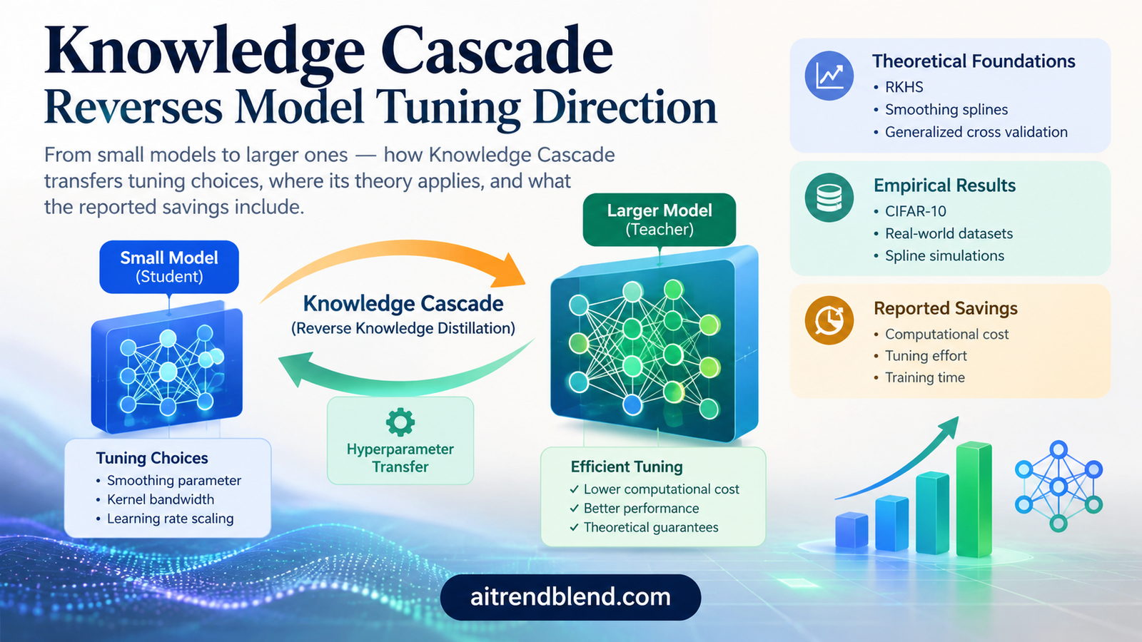
An analyst waits for another smoothing parameter search to finish. Each candidate requires an expensive fit on the same large dataset, and several candidates have already been rejected. A small pilot fit could have tested those choices much more cheaply. Knowledge Cascade asks whether the pilot can do more than suggest a starting point. With the right scaling law, it can supply the full model’s tuning choice.
- Knowledge Cascade transfers information from a cheaper student model to a larger teacher model.
- The main method tunes smoothing parameters on a subsample and scales them for a final fit on all observations.
- The strongest theory concerns nonparametric estimation in reproducing kernel Hilbert spaces.
- Kernel density bandwidth transfer follows a different scaling rule, while neural network learning rate transfer is evaluated empirically.
- The reported savings concern a development workflow, and final teacher fitting remains part of the cost.
- Biological dataset experiments do not establish diagnostic accuracy or clinical readiness.
This article explains published research. It is not medical advice, diagnosis or treatment. Consult a qualified health professional about personal care. No medical reviewer was supplied. The paper includes biological data analysis but does not validate a clinical decision system.
A small model can guide the expensive model
Luyang Fang, Haoran Lu, Yongkai Chen, Wenxuan Zhong and Ping Ma, all from the University of Georgia’s Department of Statistics, introduce the method in Knowledge Cascade, published in JMLR. The paper appears in volume 27 as article 54 in 2026. Its central question is how to reduce the cost of developing a large model before that model is fully trained.
Ordinary knowledge distillation begins with a capable teacher and transfers information into a smaller student. That arrangement can reduce deployment cost, but somebody has already paid to develop the teacher. Knowledge Cascade reverses the direction of useful guidance.
The student does not need to approximate every function the teacher can represent. It needs to recover a transferable property of the problem. In the main construction, that property is a collection of smoothing choices and the unknown constants behind their sample size scaling.
This gives the paper a distinct place in the Knowledge Distillation collection within Machine Learning. The main outcome is cheaper model development through hyperparameter transfer. It is not a claim that a smaller model becomes a more knowledgeable predictor than a larger model.
What reverse knowledge distillation means here
The phrase can invite the wrong mental picture. There is no requirement that the teacher imitate the student’s probabilities, hidden features or mistakes. The teacher receives configuration information and then learns from the full training sample.
That distinction separates KCas from a conventional distillation loss with soft targets. Our explanation of knowledge distillation mathematics describes the familiar teacher output matching objective. KCas instead treats a small model as a statistical pilot for selecting expensive training choices.
The terms student and teacher also have a precise interpretation in the spline setting. By the representer theorem, the fitted function can use one kernel section for each training observation. Fitting on fewer observations therefore changes the size of the representation, even when the underlying function space is the same.
A subsample student is cheaper partly because it has fewer data dependent basis elements. A full sample teacher retains the richer representation. The method therefore transfers a tuning decision across both sample size and effective model complexity.
The bottleneck is repeated smoothing parameter selection
Nonparametric estimation balances fitting the observations against keeping the fitted function sufficiently smooth. Too much smoothing erases structure. Too little smoothing allows a model to chase fluctuations that do not generalize.
The loss describes agreement with the data, while the penalty measures roughness. In a multivariate model, different function components can also receive different weights. The analyst may need to tune a global smoothing level and several relative component weights.
The paper uses a functional ANOVA decomposition. Main effects describe how individual coordinates contribute, and interaction terms describe joint variation. Removing higher order interactions can make the model more manageable, but it also imposes a modeling restriction.
Generalized cross validation and related criteria select smoothing parameters by repeatedly evaluating candidate fits. In the paper’s computational discussion, these searches can require matrix operations whose cost grows cubically with sample size. Repeating them for many smoothing components becomes the central bottleneck.
For Gaussian regression, the familiar GCV criterion is appropriate. For nonquadratic exponential family losses and density estimation, the authors use established variants and collectively refer to them as GCV. That shorthand should not be read as meaning every experiment uses the identical numerical objective.
The student estimates a constant that the teacher cannot know directly
The transfer begins with a statistical scaling relationship. In the initial smoothing spline illustration, an asymptotically optimal regularization level has a sample size power multiplied by an unknown constant. That constant depends on the target function, so it is unavailable as an oracle input.
The parameter controlling the smoothness order is distinct from the parameter describing additional regularity of the target. The paper denotes them by \(m\) and \(p\), with the latter lying between one and two. Neither symbol denotes the number of predictors in this formula.
The student estimates its smoothing parameter from the subsample. Multiplying by the appropriate sample size factor then transfers the estimated constant to the full sample regime. The method copies the relative component weights directly under the assumption that their useful proportions remain stable.
This is the part that turns subsample tuning into more than naive reuse. A small sample typically requires a different smoothing level from a large sample. Copying the student’s global regularization without scaling would ignore that change.
The final operation is still a teacher fit on all observations. The student does not replace that fit. Its contribution is to avoid repeatedly solving the expensive full sample problem while searching for tuning parameters.
The transferable knowledge is a scale adjusted configuration. The teacher keeps the full dataset and its larger representation, while the student supplies a cheaper estimate of how strongly that representation should be regularized.
The exponent is an assumption worth checking
In their experiments, the authors use smoothness order two and the additional regularity choice two. These imply an exponent of four ninths for the smoothing parameter transfer. The paper describes this as an empirical choice for the studied settings.
An application with a rougher target need not support the same choice. The transfer rule is only as appropriate as the relationship used to move between scales. A different smoothness regime changes the exponent and can change the full sample regularization materially.
Uniform sampling is used to construct the student. That is simple and inexpensive, but a pilot can miss uncommon regions of a distribution. A global scaling adjustment cannot reconstruct structure the student never had enough information to identify.
The practical spline simulations use a subsample size proportional to the fourth root of the full size, with a multiplier of 50. The asymptotic fourth root description alone is not a complete recipe for small datasets. The proportionality constant and the requirement that the subsample not exceed the available data still matter.
An applied analyst should therefore inspect variation across pilot draws and sensitivity to the exponent. Those are suggested diagnostics, not additional experiments reported in the paper. They help determine whether a seemingly cheap transfer is stable enough to replace a full tuning search.
What the spline theorems establish
The density and regression results control an estimation error measured through a combination of a variance related metric and the roughness penalty. The bound has one term describing stochastic error and another describing regularization bias.
The theorems assume regularity conditions involving the function space, eigenvalues, smoothness, local curvature and moments. They also require the student’s smoothing parameter to shrink at a suitable rate as the student sample grows.
The absence of an explicit predictor dimension from the displayed rate is not a free removal of dimensional difficulty. The paper states that its dimensionless formulation incorporates smoothness assumptions whose demands become stronger as dimension grows. That qualification belongs alongside the result.
The regression theorem addresses exponential family estimation in the stated spline setting. It does not certify a learning rate scaling law for an arbitrary neural architecture. The paper explicitly separates that empirical extension from the RKHS based guarantees.
A useful reading is that KCas preserves a favorable estimation regime when the student information and scaling assumptions are appropriate. It does not prove that every subsample selected configuration is optimal at every larger sample size.
Kernel density estimation uses another scaling law
The univariate kernel density example gives a particularly clear view of the principle. A Gaussian kernel estimator averages a small density bump around each observation. Its bandwidth controls the smoothness of the resulting density.
The classical asymptotic bandwidth contains a constant involving the unknown density’s curvature. The student estimates a bandwidth from a subset, and the teacher receives that bandwidth multiplied by the appropriate ratio power.
The KDE simulations compare several base selectors, including Silverman’s rule, improved Sheather Jones selection and least squares cross validation. KCas inherits important properties of the selector it uses. A scaling relationship does not make a normal reference rule equally suitable for all multimodal densities.
The study considers six univariate density shapes, sample sizes from 200 to 5000 and 50 replications. Its KCas versions use a subsample of 200 observations. The authors report that the structured plug in variants tend to be more stable than the cross validation variant in their tested settings.
The oracle bandwidth comparison is a simulation reference based on the known generating density. It is not a usable option for an ordinary dataset. Nor should an asymptotically motivated oracle benchmark be treated as a universal mathematical lower bound on every possible finite sample density estimate.
Tuning becomes cheaper while final fitting remains
The paper describes a reduction in the repeated smoothing search from a full sample cubic cost to a subsample cubic cost. With a fourth root subsample size, the sample size exponent of that tuning component becomes three quarters.
The word component is essential. After selecting the parameters, the teacher still needs to fit on the full sample. Its memory requirements and linear algebra do not disappear. Density estimation may also require numerical integration and repeated optimization even with fixed parameters.
This distinction helps explain why a large asymptotic reduction in tuning work need not produce the same reduction in total runtime. The gain depends on how much of the original workflow was spent searching, how many searches are avoided and how expensive the final solve remains.
The same care applies to neural experiments. If a student is already available, its cost can reasonably be treated as previously incurred for an incremental decision. If it is trained solely for the cascade, its development cost belongs in the total budget.
KCas makes the search cheaper. Evaluate total development cost as student tuning plus parameter transfer plus final teacher fitting, and state clearly whether the student already existed.
The simulation timings show a real tradeoff
The smoothing spline simulations compare full sample GCV with KCas and several alternatives. These include a subsample procedure, a main effects model, an order based regularization choice and a shortcut procedure for regression.
The most difficult reported regression timing setting uses 20 predictor dimensions. The table below preserves the paper’s median times in minutes. Faster alternatives exist, so the claim is a balance between estimation quality and cost rather than winning every runtime column.
| Sample size | Full GCV | KCas | Main effects GAM | Subsample method | Order based | Shortcut SKIP |
|---|---|---|---|---|---|---|
| 5000 | 42.2 | 6.1 | 1.3 | 5.5 | 16.2 | 2.1 |
| 10000 | 72.9 | 9.4 | 2.5 | 7.0 | 23.1 | 3.3 |
| 20000 | 102.5 | 8.1 | 3.2 | 5.0 | 30.8 | 3.5 |
All spline simulation results are based on 30 replications. The associated error plots compare against each replication’s full GCV estimate. Negative values of the log relative error indicate that a method did better than that reference for that replication.
Doing better than full GCV is possible because a data driven tuning rule is not an oracle. A transferred choice can behave differently from the full sample search and sometimes generalize better. The paper discusses possible explanations, but does not establish a general theorem that less tuning data improves prediction.
Real datasets do not show a universal accuracy improvement
The real data spline studies split observations into 80 percent training and 20 percent testing. Continuous features are scaled using transformations fitted on the training data. Density estimation is evaluated by test log likelihood, while regression uses relative mean squared error.
KCas performs strongly against the reported computational alternatives, but its comparison with full GCV varies by dataset. Table 3 reports relative MSE values of 0.7963 for SUSY, 1.0434 for wall following robot navigation, 0.9999 for occupancy, 0.9825 for shill bidding and 1.0040 for the CIFAR regression task.
A value above one means worse MSE than the full GCV reference. Thus the navigation and CIFAR rows should not be presented as accuracy wins over full GCV. They can still represent useful compromises when the computational savings matter.
The SUSY dataset has a much larger original size, but the paper uses 20000 sampled observations as its full sample for this comparison because the unrestricted GCV computation is unaffordable. The reported result is not an evaluation of full spline GCV on all five million observations.
There are also two different CIFAR experiments. The regression table uses extracted features and a binary automobile versus other classes task. The later deep learning study uses ten class image classification. Their metrics should not be merged into one result.
Biological datasets require a narrow interpretation
The density benchmarks include CD14 data with 13 protein measurements across 2096 cells and mouse embryonic stem cell data using four features for 1027 genes. These are biological estimation tasks, which is why the article includes the research information notice.
For CD14, the reported relative test log likelihood is 0.9998 and relative computational time is 0.86 against full GCV. For the stem cell dataset, those values are 1.0475 and 0.53. The table reports likelihood ratios as its comparison measure. These numbers are not diagnostic accuracy, patient risk estimates or clinical effect sizes.
The biological sample units also matter. Cells and genes are not patients, and a count of cellular observations does not establish independent clinical validation across people. The paper does not report a patient level prediction endpoint for these density experiments.
Clinical translation gap
A faster method for selecting smoothness may help a biomedical analysis workflow, but clinical deployment would require a defined clinical target, an appropriate study population and validation of that target. None is supplied by a benchmark density likelihood alone.
Sampling assumptions deserve attention in any later application. Related cells, repeated measurements or batch effects could affect the relationship between a small pilot and a full dataset. This is an application concern inferred from the method’s transfer mechanism, not a demonstrated failure in the paper.
The study does not establish subgroup clinical sensitivity, external hospital performance or safety of treatment decisions. Those are absent endpoints rather than disappointing scores. Our related discussion of knowledge distillation and medical model explanations concerns a different evidence question and does not supply missing clinical validation for KCas.
The neural network extension transfers learning rates
The image experiment uses MobileNetV2 and ResNet18 as students and ResNet50 as the teacher. The paper reports model sizes of 2.2 million, 11.7 million and 25.6 million parameters respectively. The architectures are adapted for the image resolution by changing the initial convolution and removing the initial max pooling.
Student grid search evaluates 12 combinations of batch size, learning rate and weight decay. Training runs for 200 epochs with stochastic gradient descent, cosine decay and a warmup covering five percent of the schedule. A holdout validation fraction of ten percent selects the configuration.
The full teacher retuning baseline evaluates 36 combinations. KCas instead transfers the student’s selected learning rate according to a batch size ratio, using either linear scaling or the square root of that ratio.
The authors report competitive teacher performance and somewhat more stable behavior for the square root option in this experiment. The spline theorem does not prove either neural scaling choice. Architecture, batch size, optimizer behavior and training dynamics can all affect transfer.
| Student architecture | Student time in hours | KCas time in hours | Cookbook time in hours | Full retuning time in hours |
|---|---|---|---|---|
| MobileNetV2 | 3.5 | 6.9 | 3.4 | 121.1 |
| ResNet18 | 18.5 | 21.8 | 3.4 | 121.1 |
These are the median computational times in Table 5. Accuracy comparisons are plotted and summarized over three repetitions, without a table of precise final accuracy values. This article therefore does not invent decimal accuracy scores from the figure.
The stronger student costs more to develop and provides more useful guidance in the reported comparison. That creates a practical decision. Choosing the cheapest possible student may reduce the tuning bill while weakening the transferred information. Our article on distillation across forecasting architectures offers a separate example of why architecture and transfer direction should be specified, though its results do not validate the KCas learning rate rule.
Limitations worth retaining in any implementation
The unknown scaling relationship is the central dependency. In the spline case, smoothness and eigenvalue conditions provide the justification. In the neural case, empirical observations motivate the rule. A model developer should not flatten those into a single universal guarantee.
The pilot must capture relevant structure, including interaction balance. Directly copying relative component weights assumes that the small sample identifies useful proportions. Rare regions or a poorly chosen subsample can challenge that assumption even when the final teacher sees every observation.
The reported real datasets and architecture pairs cover useful but limited settings. They do not establish performance for every optimizer, model family, data regime or compute platform. Hardware specific runtime measurements also do not directly establish energy savings or monetary savings elsewhere.
For the biological examples, sample diversity, batch structure and generalization to an intended clinical population would need separate study. No prospective evaluation, diagnostic operating point or clinical uncertainty analysis is reported. There is no basis for claiming a clinically approved system from these results.
Finally, the scope of the final fit can still be the bottleneck. KCas does not by itself remove a dense kernel matrix or make an otherwise impossible full sample teacher fit feasible. It removes repeated tuning work when that work is a meaningful portion of the development budget.
“the student does not need to learn everything the teacher will eventually learn”Fang, Lu, Chen, Zhong and Ma, explaining the information transfer principle.
A pilot becomes useful when its scaling is credible
Knowledge Cascade gives a concrete answer to a practical question. A small preliminary model can guide a larger model without first matching all of its predictive ability. In the main setting, it estimates smoothing information that would be expensive to tune at full scale.
The conceptual change is the purpose assigned to the student. It becomes a source of configuration knowledge for model development. The teacher remains responsible for the final function estimate on the complete training sample.
The most convincing transfer is supported by a justified relationship between sample size and tuning level. Spline regularization and classical KDE bandwidths provide explicit examples. Learning rate transfer extends the same idea empirically, with a more limited basis for generalization.
The experiments support favorable computational compromises, including settings where KCas matches or exceeds full GCV. They also show slower alternatives, accuracy tradeoffs and the cost of obtaining a stronger student. Keeping those details visible makes the method more useful to practitioners.
Future work can test transfer stability across pilot draws, learn appropriate scaling relationships and broaden the architectures and datasets studied. The immediate lesson is actionable. Before repeating an expensive search, identify which part of its answer a small model could estimate reliably.
Complete PyTorch reference for a spline specialization
The reference implements periodic cubic spline ANOVA regression with Gaussian responses. It provides a custom kernel, a full fitted model, the penalized objective, exact linear smoothing fits, finite GCV search, student sampling, smoothing parameter transfer, teacher fitting, evaluation and a runnable synthetic smoke test. A second example implements the Silverman KDE transfer rule.
The periodic kernel has a constant unpenalized component, main effects and pair interactions. The search uses a small collection of interaction weight profiles, rather than estimating every component weight from the paper. Exact spectral calculations replace iterative neural training because the Gaussian specialization permits a direct solution.
This is an independent educational implementation. It does not reproduce the paper’s nonperiodic spline package, density likelihood optimization, generalized approximate cross validation, term diagnostics or neural network grid searches. The demonstration subsample size and search grid are explicit implementation choices.
The code reuses a matrix factorization across candidate smoothing values within each profile. Its operation counts therefore differ from a workflow that refits every candidate independently. It records student selection time separately from teacher fitting time and makes no claim to reproduce published speedups.
Python syntax and independent numerical checks passed. PyTorch was unavailable in the execution environment, so the runtime smoke test remains unexecuted. No benchmark score or training success is claimed from this code.
"""Educational Knowledge Cascade specialization, JMLR 27(54), 2026.
Periodic cubic spline ANOVA kernel + Gaussian regression + exact linear GCV.
Independent PyTorch code, not the authors' package or benchmark reproduction.
No iterative optimizer needed: each Gaussian fit is a closed-form solve.
CPU float64. Run this file for synthetic checks and a small demonstration.
"""
import math
import time
import torch
from torch import nn


class PeriodicCubicANOVA(nn.Module):
    """Normalized periodic cubic Sobolev kernel, main and pair effects.

    k(t) = -30 B4(frac(t)), B4(t)=t^4-2t^3+t^2-1/30.
    Normalization changes penalty scale, not the smoothness order m=2.
    The unpenalized null space is a constant. No nonperiodic linear terms.
    """
    def __init__(self, dimension, interaction_weight):
        super().__init__()
        if dimension < 1 or interaction_weight < 0:
            raise ValueError('Require positive dimension and nonnegative weight')
        self.dimension = dimension
        self.interaction_weight = float(interaction_weight)

    def forward(self, x, z):
        if x.shape[1] != self.dimension or z.shape[1] != self.dimension:
            raise ValueError('Incorrect number of covariates')
        difference = torch.remainder(x[:, None, :] - z[None, :, :], 1.)
        components = -30 * (difference**4 - 2*difference**3 +
                            difference**2 - 1/30)
        result = components.sum(dim=-1)
        for j in range(self.dimension):
            for k in range(j + 1, self.dimension):
                result = result + self.interaction_weight * components[..., j] * components[..., k]
        return result


class SplineModel(nn.Module):
    def __init__(self, kernel, centers, coefficients, intercept):
        super().__init__()
        self.kernel = kernel
        self.register_buffer('centers', centers.clone())
        self.register_buffer('coefficients', coefficients.clone())
        self.register_buffer('intercept', intercept.clone())

    def forward(self, x):
        return self.intercept + self.kernel(x.double(), self.centers) @ self.coefficients


def center_matrix(k):
    return k - k.mean(0, keepdim=True) - k.mean(1, keepdim=True) + k.mean()


def gaussian_objective(model, x, y, regularization):
    """mean squared residual + lambda times RKHS squared seminorm."""
    c = model.coefficients
    k = model.kernel(model.centers, model.centers)
    penalty = c @ k @ c
    return (y - model(x)).square().mean() + regularization * penalty


@torch.no_grad()
def spectral_setup(kernel, x, y):
    k = kernel(x, x)
    kc = center_matrix(k)
    eigenvalues, eigenvectors = torch.linalg.eigh((kc + kc.T) / 2)
    # Clamp only roundoff-level negative eigenvalues; reject a bad kernel.
    if eigenvalues.min() < -1e-8 * max(1., eigenvalues.max().item()):
        raise RuntimeError('Kernel is not numerically positive semidefinite')
    eigenvalues = eigenvalues.clamp_min(0)
    centered_y = y - y.mean()
    transformed_y = eigenvectors.T @ centered_y
    return k, eigenvalues, eigenvectors, transformed_y


@torch.no_grad()
def fit_at_lambda(kernel, x, y, regularization, setup=None):
    if regularization <= 0:
        raise ValueError('regularization must be positive')
    if setup is None:
        setup = spectral_setup(kernel, x, y)
    k, values, vectors, uy = setup
    n = len(x)
    coefficients = vectors @ (uy / (values + n * regularization))
    # Explicit null-space constraint removes floating-point constant residue.
    coefficients = coefficients - coefficients.mean()
    intercept = y.mean() - k.mean(0) @ coefficients
    model = SplineModel(kernel, x, coefficients, intercept)
    fitted = model(x)
    degrees = 1 + (values / (values + n * regularization)).sum().item()
    denominator = 1 - degrees / n
    if denominator <= 1e-10:
        raise RuntimeError('Degenerate GCV denominator')
    gcv = (y - fitted).square().mean().item() / denominator**2
    # Stationarity of (K+n*lambda*I)c + b*1 = y.
    residual = k @ coefficients + n * regularization * coefficients + intercept - y
    relative = torch.linalg.vector_norm(residual) / (1 + torch.linalg.vector_norm(y))
    if relative > 1e-7:
        raise RuntimeError('Spline normal equations failed')
    return model, {'gcv': gcv, 'degrees_of_freedom': degrees,
                   'relative_normal_residual': relative.item()}


@torch.no_grad()
def select_student(x, y, grid, profiles=(0., 0.3, 1.)):
    """Finite search, reusing each profile's factorization across lambdas.

    Profiles tune a single pair-effect weight, not every paper theta.
    Uses ordinary GCV only; no GACV, density likelihood or term diagnostics.
    """
    best = None
    for profile in profiles:
        kernel = PeriodicCubicANOVA(x.shape[1], profile)
        setup = spectral_setup(kernel, x, y)
        for value in grid:
            regularization = float(value)
            model, report = fit_at_lambda(kernel, x, y, regularization, setup)
            if best is None or report['gcv'] < best['report']['gcv']:
                best = {'model': model, 'lambda': regularization,
                        'profile': profile, 'report': report}
    best['factorizations'] = len(profiles)
    best['lambda_evaluations'] = len(profiles) * len(grid)
    return best


def transfer_lambda(student_lambda, n, b, m=2., smoothness=2.):
    if not (0 < b <= n and student_lambda > 0 and m > 0 and 1 <= smoothness <= 2):
        raise ValueError('Invalid transfer parameters')
    return student_lambda * (n / b)**(-2*m / (2*m*smoothness + 1))


@torch.no_grad()
def train_cascade(x, y, b=64, seed=5):
    x, y = x.double(), y.double()
    n = len(x)
    if not 2 < b <= n or y.shape != (n,) or not torch.isfinite(x).all() or not torch.isfinite(y).all():
        raise ValueError('Invalid finite training data or subsample size')
    generator = torch.Generator().manual_seed(seed)
    indices = torch.randperm(n, generator=generator)[:b]
    grid = torch.logspace(-6, 0, 25, dtype=x.dtype)
    start = time.perf_counter()
    student = select_student(x[indices], y[indices], grid)
    tuning_seconds = time.perf_counter() - start
    teacher_lambda = transfer_lambda(student['lambda'], n, b)
    kernel = PeriodicCubicANOVA(x.shape[1], student['profile'])
    start = time.perf_counter()
    teacher, report = fit_at_lambda(kernel, x, y, teacher_lambda)
    fitting_seconds = time.perf_counter() - start
    return teacher, {'student_lambda': student['lambda'],
                     'teacher_lambda': teacher_lambda,
                     'interaction_weight': student['profile'],
                     'student_size': b, 'teacher_size': n,
                     'student_tuning_seconds': tuning_seconds,
                     'teacher_fitting_seconds': fitting_seconds,
                     'student_factorizations': student['factorizations'],
                     'teacher_factorizations': 1,
                     'student_lambda_evaluations': student['lambda_evaluations'],
                     'teacher_report': report,
                     'scope': 'periodic Gaussian specialization; no benchmark claim'}


@torch.no_grad()
def evaluate(model, x, y):
    return {'mse': (model(x.double()) - y.double()).square().mean().item()}


class GaussianKDE(nn.Module):
    """A second, exact KCas-Silverman illustration for univariate KDE."""
    def __init__(self, observations, bandwidth):
        super().__init__()
        if bandwidth <= 0:
            raise ValueError('Require positive bandwidth')
        self.register_buffer('observations', observations.double().reshape(-1))
        self.bandwidth = float(bandwidth)

    def forward(self, points):
        u = (points.double().reshape(-1, 1) - self.observations) / self.bandwidth
        return torch.exp(-u.square()/2).mean(1) / (self.bandwidth * math.sqrt(2*math.pi))


def silverman_bandwidth(x):
    scale = min(x.std(unbiased=True).item(),
                (torch.quantile(x, .75)-torch.quantile(x, .25)).item()/1.34)
    if scale <= 0:
        raise ValueError('Degenerate scale; no silent bandwidth replacement')
    return .9 * scale * len(x)**(-.2)


def true_function(x):
    return torch.sin(2*math.pi*x[:, 0]) + .5*torch.cos(2*math.pi*x[:, 1]) + \
           .4*torch.sin(2*math.pi*x[:, 0])*torch.cos(2*math.pi*x[:, 1])


def smoke_test():
    torch.manual_seed(42)
    x = torch.rand(256, 2, dtype=torch.float64)
    y = true_function(x) + .1*torch.randn(256, dtype=torch.float64)
    test_x = torch.rand(128, 2, dtype=torch.float64)
    model, report = train_cascade(x, y, b=64)
    assert model(test_x).shape == (128,)
    assert math.isfinite(gaussian_objective(model, x, y, report['teacher_lambda']).item())
    assert report['teacher_lambda'] < report['student_lambda']
    assert transfer_lambda(.1, 64, 64) == .1
    assert abs(transfer_lambda(.1, 576, 64)/.1 - 9**(-4/9)) < 1e-12
    print({'settings': report, 'noiseless_test': evaluate(model, test_x, true_function(test_x))})
    observations = torch.randn(512, dtype=torch.float64)
    subsample = observations[torch.randperm(512)[:200]]
    h_sub = silverman_bandwidth(subsample)
    h_full = h_sub * (len(observations)/len(subsample))**(-.2)
    kde = GaussianKDE(observations, h_full)
    grid = torch.linspace(-8, 8, 4096, dtype=torch.float64)
    mass = torch.trapz(kde(grid), grid).item()
    assert abs(mass-1) < .001
    print({'kde_mass_on_grid': mass, 'bandwidth': h_full,
           'notice': 'educational run, not the paper experiments'})


if __name__ == '__main__':
    smoke_test()
Frequently asked questions
What is Knowledge Cascade?
It is a framework that transfers useful information from a cheaper student model to a larger teacher model. In the main spline setting, the transferred information is a collection of smoothing parameters adjusted for sample size.
Does the teacher copy the student’s predictions?
That is not required by the method studied here. The student supplies configuration information, and the teacher still fits the final function using all training observations.
Why must the smoothing parameter be scaled?
Its appropriate value changes with sample size. Knowledge Cascade estimates a problem dependent constant from the student and transfers it using a specified statistical scaling relationship.
Does KCas remove the cost of fitting the teacher?
No. It reduces repeated tuning work. The final full sample teacher fit, its memory requirements and the cost of developing the student remain relevant to the total budget.
Do the spline theorems guarantee neural learning rate transfer?
No. The main guarantees concern the stated nonparametric function spaces and regularity conditions. Linear and square root learning rate scaling are evaluated empirically in the image classification experiment.
Do the biological experiments establish clinical readiness?
No. They evaluate density estimation on cellular and gene related measurements. They do not establish diagnostic accuracy, patient benefit or clinical deployment safety. The independent PyTorch reference also has no clinical validation.
Read the paper and inspect the reference
The publisher provides the full paper and links the authors’ repository. The independent PyTorch reference printed here is a separate Gaussian regression specialization.
Luyang Fang, Haoran Lu, Yongkai Chen, Wenxuan Zhong and Ping Ma. Knowledge Cascade. Reverse Knowledge Distillation on Nonparametric Multivariate Functional Estimation. Journal of Machine Learning Research, volume 27, article 54, pages 1 to 38, 2026. Formal title punctuation normalized for this article’s prose style.
This analysis is based on the published paper and an independent evaluation of its claims.