
- Clinical information fusion
- Missing modalities
- Equiangular tight frame
- Neural collapse
- ICU mortality
- MIMIC-IV and eICU
- PyTorch
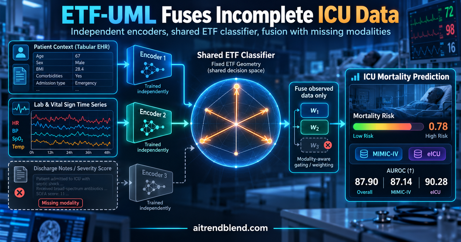
It is the middle of a night shift in an intensive care unit. One patient has a full set of overnight labs and a running stream of vital signs. The patient in the next bed has demographics and diagnosis codes on file, but the lab panel was never ordered because nobody thought it was needed. The discharge summary for either of them will not exist until the day they leave. Any risk model running on that ward sees a different collection of data for every patient, and a different collection again for the same patient a few hours later.
A team at Yonsei University, JaeSeong Hong, Mingyu Kim and Yu Rang Park, built ETF-UML for exactly that situation. Instead of training one big network on all the data sources together, it trains each source’s encoder on its own and keeps them compatible by aiming all of them at the same fixed geometric target, borrowed from the theory of neural collapse. The fusion step then combines whatever happens to be present.
Key points
- ETF-UML trains a separate encoder for coded patient context, lab and vital trajectories, and notes or severity scores, each against one shared and frozen equiangular tight frame classifier.
- A small gate weights only the observed modalities using how much data each has and how long the patient has been admitted, and the prototypes are adjusted only during the first 10 fusion epochs.
- On MIMIC-IV 30 and 90 day mortality and eICU 10 day mortality, it has the highest mean AUROC and AVG of 12 compared methods. MUSE keeps the best AUPRC on eICU.
- Sharing and fixing the target is what makes composition work. Without either property, simple averaging of the encoders drops the 90 day AVG from 65.89 to about 38 to 40.
- For two class tasks we show the shared geometry reduces to one fixed decision axis, which explains why it works and why it breaks when the prototypes differ.
- All evidence comes from two US critical care databases with three training seeds. No external validation, calibration analysis or subgroup analysis is reported.
Please read. This article explains published research on predicting mortality from hospital records. It is not medical advice, diagnosis, or treatment, and ETF-UML is a research method rather than a clinical tool. Decisions about care should always involve qualified clinicians.
Why missing data is the normal case in hospitals
Clinical prediction papers often treat missing data as a nuisance to be imputed away. Anyone who has worked with an electronic health record knows that is the wrong mental model. A lab result is missing because a physician decided not to order it, which says something about how sick the patient looked. Vitals are charted at intervals set by protocol and acuity. Notes are written when someone has time or when a milestone such as discharge forces it. The authors lean on prior work showing that missingness in these systems is often informative, which is a polite way of saying the gaps carry signal.
That creates two problems for multimodal models. The first is obvious. At prediction time the model sees an incomplete and shifting subset of sources. The second is subtler. Most multimodal architectures train their encoders, fusion layer and classifier together on whatever combinations appear in the training data. Representations tuned for one co occurrence pattern may not transfer to another. A model trained mostly on patients who had labs, vitals and a note may behave strangely on a patient who has only the coded context.
There is also a known failure in jointly trained multimodal networks called modality collapse, where the shared representation leans on whichever source contributes most to the loss and quietly neglects the rest. Methods such as MCR, from Kontras and colleagues, try to regularise that competition, but they still train everything jointly.
ETF-UML takes a deliberately conservative position. It does not try to impute the missing sources, it does not model the arrival process over time, and it does not train the encoders together. It asks a narrower question. Can encoders that never see each other during training still be combined reliably afterwards?
What earlier methods do with missing modalities
The paper groups prior work into three families, and it is worth seeing where each one leans. Imputation methods fill the gaps. GRAPE treats patients and features as a bipartite graph and propagates information from observed to missing features. OmniFuse imputes embeddings for any missing combination and weights each modality by how confidently the rest already predict the label. Both add a generative objective and assume the missing information can be recovered from what is present, which is exactly the assumption that informative missingness undermines.
Robust training methods avoid imputation. SMIL uses Bayesian meta learning to adapt at inference when some modalities are absent, at the cost of episodic training and a dependence on stable co occurrence patterns. Disentanglement methods split representations into shared and modality private parts. ShaSpec factorises features this way with alignment on the shared part. M3Care adds a patient similarity objective anchored on patients who have every modality. MUSE builds patient to modality bipartite graphs and propagates across both, handling missing labels as well. DERL routes each modality through private and shared experts with reconstruction objectives.
The common thread, as the authors put it, is joint multimodal optimisation. Every one of these needs modalities to be co observed during training, either for an alignment loss or for a fusion loss. If you have read our analysis of MADAT and missing multimodal data in prognosis, you will recognise the same dependence. ETF-UML’s bet is that you can drop it entirely if the encoders agree on what the decision should look like before any of them starts training.
Neural collapse, and why a fixed classifier helps
Neural collapse is an observation from the late phase of training deep classifiers. Papyan and colleagues found that class mean features and the classifier’s weight vectors drift toward a very specific arrangement called a simplex equiangular tight frame. In that arrangement every class prototype has the same length, every pair is separated by the same angle, and together they spread out as far as geometry allows. Later theory from Zhu and colleagues showed this configuration is a global optimum for common classification losses under simplified feature models.
If networks end up there anyway, why not start there? Fixed ETF classifiers do exactly that. The classifier is set to the simplex shape and frozen, so the encoder only has to pull each class’s features toward a known direction. Yang and colleagues found this helpful for imbalanced data, and Li and colleagues used it in federated learning, where every client shares one frozen ETF so that local classifiers cannot drift apart.
Here is where it gets interesting. Federated clients and hospital data sources have something in common. Both are trained separately and need to agree afterwards. ETF-UML transfers the federated trick to modalities. Each encoder is a client, and the shared frozen ETF is the contract that keeps them compatible.
How ETF-UML is built
Building the shared target
The prototypes are built once, before any training. A random Gaussian matrix \(R \in \mathbb{R}^{d\times C}\) is factorised by QR decomposition to get an orthonormal basis \(Q\), and the simplex ETF follows.
The embedding dimension is \(d = 1536\) and \(C\) is the number of classes, two for the mortality tasks. The matrix stays frozen for the whole unimodal stage.
Training each modality alone
For modality \(m\), an encoder \(f_m\) and projection head \(p_m\) map the input to a unit length vector, and the logits are scaled dot products with the shared prototypes.
Each encoder is trained independently with the balanced softmax loss of Ren and colleagues, which adds the log class prior to the logits during training to counter class imbalance. There is no cross modal alignment term at all. That absence is intentional. A paired alignment loss would need patients who have both modalities, and would tilt the representation toward that subgroup. With ETF-UML, each encoder trains on every patient who has its modality.
The architectures follow the MUSE benchmark. Tabular context uses a multilayer perceptron, lab and vital trajectories use a Transformer or GRU, and discharge notes use TinyBERT.
Fusing only what is there
Once the encoders are trained, they are frozen. For each observed modality, a small metadata vector \(u^{(m,t)}\) records two things, the acquisition size, meaning how many events were recorded, and the time since admission. Each modality has its own three layer perceptron with a hidden width of 16 that turns that metadata into a score, and a softmax over the observed modalities only turns scores into weights.
Missing modalities get no weight and no say. The idea of a gate that weighs sources case by case is familiar from mixture of experts fusion of skin images and patient metadata, and from LGFN, which reroutes when polarization sensors are unavailable. What is different here is that the gate only ever sees acquisition context, never the data itself. The fused vector goes through the same scaled dot product with \(V\), and the fusion stage minimises balanced softmax loss over the gates, the scale and, briefly, the prototypes.
A short window for adjusting the target
The fused vectors live in a slightly different distribution from any single modality, so the authors let \(V\) move during the first 10 of 100 fusion epochs and then freeze it again. They frame this as calibration rather than redesign, and they check afterwards that the prototype pair stays antipodal and rotates by less than 0.4 degrees.
The encoders never meet during training. They agree because they were all told, in advance and in the same words, what the answer should look like. aitrendblend analysis of ETF-UML, Information Fusion 2027
What the shared geometry really is when there are two classes
This is not a small distinction, and the paper does not spell it out. For the mortality tasks \(C = 2\), so Equation 1 produces just two vectors. Work through the algebra and they come out as \(v_0 = (q_0 – q_1)/\sqrt{2}\) and \(v_1 = -v_0\), two unit vectors pointing in exactly opposite directions. The logit difference then reduces to a single projection.
In other words, in a 1536 dimensional space, the entire decision depends on one fixed direction. Every encoder, trained alone, is pushed to place survivors on one side of that line and deaths on the other. Everything else in the embedding is free to do whatever it likes.
That reading explains several results at once. The inter modality cosine between class centre directions is between 0.960 and 0.973, and the cosine between those directions and the prototype axis is at least 0.980 on every task. Of course it is. Every encoder was trained to align with the same axis. It also explains why the embedding dimension barely matters. On 30 day mortality the AVG for 512, 1024 and 1536 dimensions differs by less than 0.06, since only one direction carries the supervised signal.
Most usefully, it explains Table 3 of the paper. If each encoder gets its own random ETF, each learns its own decision axis, and in high dimensions random axes are nearly orthogonal. Averaging the embeddings then mixes one modality’s signal with directions that mean nothing to the others. The fused score is mostly noise, which is exactly what the uniform fusion column shows. Because the fused vector is renormalised, the final score is also a weighted average of per modality projections divided by how much the modalities disagree elsewhere, which is a quietly sensible way to sharpen a prediction when sources agree.
What the experiments show
The study follows the MUSE benchmark protocol on three ICU mortality tasks. MIMIC-IV supplies 30 and 90 day post discharge mortality with tabular context, lab and vital trajectories and discharge notes. eICU supplies 10 day in hospital mortality with tabular context, lab and vital trajectories and the APACHE score. Missingness is real, not simulated.
| Item | MIMIC-IV 30 day | MIMIC-IV 90 day | eICU 10 day |
|---|---|---|---|
| Patients | 190,027 | 164,723 | 119,852 |
| Train, validation, test | 133,018, 19,003, 38,006 | 115,306, 16,472, 32,945 | 83,896, 11,985, 23,971 |
| Positive rate | 3.37% | 9.22% | 4.64% |
| Lab and vital missing | 17.39% | 17.03% | 0.87% |
| Note or APACHE missing | 38.52% | 38.46% | 9.44% |
| Mean age | 60.96 | 61.71 | 62.95 |
Table A. Cohorts from Table 1 of Hong et al. Tabular context is fully observed in all three tasks. Missing rates are at the modality level.
Training uses the last available timepoint for each patient, and splits are at the patient level, so no person appears in more than one partition. Unimodal encoders train with early stopping at a patience of 15 and at most 100 epochs. Every method reports the checkpoint with the best validation AUROC across three seeds, 2026, 2027 and 2028.
Eleven baselines sit in the main table. Three unimodal models, three end to end fusion variants that sum, concatenate or attend over modality embeddings, and five missing modality methods, GRAPE, SMIL, M3Care, ShaSpec and MUSE. Metrics are AUROC, AUPRC and their average, called AVG. The full numbers are in the ETF-UML paper in Information Fusion, which is open access.
| Method | 30 day AUROC | 30 day AUPRC | 90 day AUROC | 90 day AUPRC | eICU AUROC | eICU AUPRC |
|---|---|---|---|---|---|---|
| Tabular only | 85.54 | 20.90 | 85.40 | 41.33 | 84.69 | 30.23 |
| Note only or APACHE only | 85.62 | 28.38 | 83.39 | 44.42 | 86.51 | 30.84 |
| End to end attention | 84.88 | 26.56 | 84.45 | 41.53 | 89.45 | 43.53 |
| GRAPE | 79.61 | 17.81 | 81.16 | 33.92 | 86.52 | 39.83 |
| ShaSpec | 84.12 | 24.80 | 84.50 | 40.73 | 88.72 | 44.72 |
| MUSE | 85.60 | 25.03 | 86.03 | 42.96 | 89.07 | 45.91 |
| ETF-UML | 87.90 ± 0.60 | 29.32 ± 1.63 | 87.14 ± 0.10 | 46.43 ± 0.30 | 90.28 ± 0.43 | 45.48 ± 3.33 |
Table B. Selected rows from Table 2 of Hong et al., means over three seeds. ETF-UML reaches AVG scores of 58.61, 66.79 and 67.88. The paper also reports Lab and Vital only, end to end sum and concat, SMIL and M3Care, all below ETF-UML on AUROC and AVG.
ETF-UML has the best mean AUROC and AVG on all three tasks and the best AUPRC on both MIMIC-IV tasks. The one exception is eICU AUPRC, where MUSE’s 45.91 edges ETF-UML’s 45.48, a difference the paired test does not call significant at a corrected q of 0.270. The closest competitors overall are MUSE and ShaSpec. Margins over MUSE in AUROC are 2.3, 1.1 and 1.2 points across the three tasks.
AUPRC needs context, because its baseline is the prevalence. A random score would get about 3.4 on 30 day mortality, 9.2 on 90 day mortality and 4.6 on eICU. ETF-UML’s AUPRC values are roughly 8.7, 5.0 and 9.8 times those floors. Still, a 30 day AUPRC of 29.32 means that at most operating points the majority of patients flagged as high risk survive. That is normal for rare outcomes and important for anyone imagining an alert system.
One more detail is worth noticing. On 30 day mortality, the discharge note alone gets an AUPRC of 28.38, within one point of the full model. In the pooled comparison across tasks, the difference against the note only model on AUPRC is the one that does not reach significance, at q equal to 0.083. Discharge notes are dense with clinical judgement, and for post discharge outcomes they carry much of the useful signal.
When the available data change
Two further experiments stress the claim that matters most, robustness to changing availability. In the pre discharge evaluation, a model trained on the final observation is tested on disjoint hourly bins before discharge, where on MIMIC-IV the note is missing by construction. Performance generally rises toward discharge as data accumulate, and ETF-UML stays competitive across bins. The authors are careful to say these curves are not forecasts, since bins are evaluated independently.
The second experiment removes modalities on purpose. Across the nine two modality subsets on the three tasks, ETF-UML has the higher AVG than MUSE in six, by 4.4 to 10.7 points in five of them, and MUSE wins the other three. Four of the nine gaps are under one point and within seed noise. One detail stands out. On 90 day mortality, dropping the tabular modality costs ETF-UML 6.6 percent of AUROC and MUSE 15.9 percent, which fits the idea that jointly trained models lean harder on whatever they saw most.
In a stress test that keeps tabular data and lowers the observation rate of the other two modalities, ETF-UML has the higher AVG in all nine settings on every task, and the gap widens as availability falls. On eICU it grows from 0.39 points with full observation to 5.34 points when both other modalities are observed only 30 percent of the time.
The headline table shows modest but consistent gains. The more persuasive evidence is the stress test, where ETF-UML’s advantage grows as data become sparser, which is the setting it was designed for.
Why the geometry matters
| Classifier during unimodal training | Tabular alone | Uniform fusion | Metadata fusion |
|---|---|---|---|
| Shared and fixed, the ETF-UML setting | 63.37 | 65.89 | 66.79 |
| Shared but learnable | 63.78 | 40.30 | 64.26 |
| Separate and fixed | 63.23 | 38.38 | 64.20 |
| Separate and learnable | 63.69 | 40.15 | 64.60 |
Table C. AVG on MIMIC-IV 90 day mortality, from Table 3 of Hong et al. Every encoder is trained independently in every row.
This is the cleanest experiment in the paper. Each encoder performs the same on its own whatever the classifier setup. But when the embeddings are averaged with equal weights, only the shared and fixed target survives. Without it, fusion falls to 38 to 40, below every single modality. The learned gate rescues most of the loss, presumably by leaning on one modality, but still trails the proposed setting by over two points. The binary axis argument above explains the collapse. If the prototype is shared but learnable, each independent training run moves it differently, and the axes stop matching.
The angle between the two prototypes matters too. Fixing them at 180 degrees gives 66.79, narrowing to 120 degrees gives 66.25, 90 degrees gives 65.20 and 60 degrees gives 60.73 with a large spread. A random angle per seed gives 64.85 with a standard deviation of 1.50, against 0.20 at 180 degrees. Training the encoders jointly instead of independently, still with the ETF, lowers the tabular model from 63.37 to 55.76 and the fused AVG to 62.48. The tabular encoder suffers most, falling by 7.61 points, against 2.21 for lab and vital and 0.73 for notes, which is a textbook sign of modality competition in joint training.
The same pattern holds on a three class task, eICU discharge destination over home, nursing facility and death. Removing either property drops uniform fusion from 69.16 to between 64.75 and 66.74, and metadata fusion recovers to between 68.56 and 69.08, below 69.25.
What each fusion component adds
| Configuration | 30 day AUPRC | 30 day AVG | 90 day AUPRC | 90 day AVG |
|---|---|---|---|---|
| No metadata, no refinement | 25.83 | 56.81 | 44.83 | 65.89 |
| Add time metadata | 26.90 | 57.16 | 44.74 | 66.26 |
| Add size metadata | 27.14 | 57.21 | 46.00 | 66.38 |
| Add prototype refinement | 29.32 | 58.61 | 46.43 | 66.79 |
Table D. Fusion ablation on MIMIC-IV from Table 5 of Hong et al. Standard deviations on AUPRC range from about 0.3 to 1.6.
Each component helps a little, and prototype refinement gives the largest single jump, most of it in AUPRC. Here is a puzzle the paper leaves open. By the binary axis argument, AUROC and AUPRC depend only on how patients are ranked along \(v_0\). Rescaling the prototypes changes confidence but not ranking. The paper reports the pair stays antipodal and rotates by less than 0.4 degrees. So the refinement gain must come either from that tiny rotation or from how the gates train while \(V\) is moving. Both are possible, and the 30 day AUPRC gain of 2.18 is only about 1.3 standard deviations. A run that refines \(V\) with the gates frozen would settle where the gain really comes from.
What the gate learns
The fusion weights are easy to read. On MIMIC-IV 30 day, with all three modalities present, they average 0.37 for tabular, 0.45 for lab and vital and 0.18 for notes. Over a stay, the tabular weight falls from 0.81 in the first six hours to 0.36 after 168 hours while the lab and vital weight rises from 0.19 to 0.62. But holding the observed set fixed on 90 day mortality, the tabular weight varies by only 0.004 across time bins. The gate mostly responds to which modalities exist, not to the clock. Increasing a modality’s acquisition size nudges its weight up, by 0.021 to 0.072 for tabular and 0.016 to 0.143 for lab and vital at 50 units depending on task.
Fused representations are also tighter. The within to between class distance ratio of the fused embedding is 0.481, 0.576 and 0.530 on the three tasks, lower than any single modality and well below MUSE’s 1.027, 1.065 and 0.548.
Cost
Because the encoders are frozen, the fusion stage is light. On MIMIC-IV 30 day it needs 31.50 GFLOPs and 0.44 of peak VRAM against 83.63 GFLOPs and 4.70 for MUSE, and 0.98 time units against 6.58. Counting the longest unimodal training run as well, assuming encoders train in parallel, ETF-UML’s total is 1.18. The table does not state units for memory or time. ETF-UML is not the cheapest in FLOPs on eICU, where the APACHE input is tiny, but it has the lowest peak memory everywhere. A practical bonus follows. Encoders can be reused across many fusion configurations without retraining, which matters in hospitals where data feeds change on different schedules.
What the paper does not settle
Three seeds measure training noise, not patient noise. Every significance test pairs three runs per task on one fixed test set. That shows the ranking is stable across random initialisations. It does not show how much the result would move with a different sample of patients. With roughly 1,281 deaths in the 30 day test set, about 3,038 in the 90 day set and about 1,112 in eICU, if prevalence matches across splits, a patient level bootstrap or DeLong test would give confidence intervals for AUROC that a clinical reader could interpret directly.
Probabilities are not risks yet. Balanced softmax trains with the class prior added to the logits, so the raw softmax at inference estimates what risk would be if deaths and survivals were equally common. For ranking metrics that does not matter. For a model that tells a clinician a patient has a 40 percent chance of dying, it matters a great deal, because the number would be inflated for rare outcomes. The paper reports no calibration curves or calibration error, and the probabilities would need correcting for prevalence before anyone read them as risks. We have written before about why models stay confident when they should not, and the same caution applies with more force at a bedside.
Informative missingness is motivated more than modelled. The introduction argues that a missing lab can carry signal. In the method, a missing modality simply gets no weight, and its metadata is not used. The absence can shift how much the remaining sources count, but it cannot by itself raise or lower a patient’s risk. A model that wanted to use the fact that no labs were ordered would need an explicit feature for it.
The binary case is a special case. Most of the geometric story is strongest with two classes, where the shared target is one axis. The three class discharge destination experiment is reassuring, but one auxiliary task is thin evidence for problems with many classes, where the ETF has more structure and independent encoders have more ways to disagree.
ETF-UML’s core idea is sound and well supported by the ablations. Before it could inform care, it would need patient level confidence intervals, prior corrected and calibrated probabilities, subgroup results and validation on a hospital outside the two benchmark databases.
Clinical translation gap
Everything here comes from MIMIC-IV and eICU, two large de identified critical care databases from US institutions, processed through one benchmark pipeline. Those databases are invaluable precisely because they are shared, and that also means models are tuned to their coding conventions, documentation styles and patient mix. A different health system codes diagnoses differently, orders labs on different thresholds and writes notes in different templates. The authors list external validation on independent cohorts as future work.
The task framing also needs thought before deployment. The MIMIC-IV tasks predict death after discharge and use the discharge note, which only exists at the moment of discharge. That is a reasonable research benchmark and a reasonable discharge planning question. It is not the same as real time deterioration prediction on the ward, and the pre discharge evaluation shows that earlier, sparser snapshots are harder.
Fairness is unexamined. Table 1 of the paper reports gender and race and ethnicity breakdowns, with about two thirds of MIMIC-IV patients recorded as Caucasian and under 3 percent as Asian, but no results are broken down by subgroup. Mortality models have a documented history of performing unevenly across groups, and documentation patterns such as note length and lab ordering can differ by group too. Since ETF-UML’s gate reacts to how much of each modality was recorded, uneven documentation could change weights in uneven ways. That deserves a direct check.
On regulation and safety, a mortality risk model used to guide individual care would generally fall under oversight for software as a medical device in most jurisdictions, requiring evidence of performance on the intended population, a clear account of intended use, and monitoring after deployment. The paper makes no such claims, which is appropriate for a methods study. Any hospital experimenting with a model of this kind should run it silently alongside clinicians first, compare its alerts with outcomes, and keep decisions with the care team.
Limitations
Sample size and statistical power. The cohorts are large, between about 120,000 and 190,000 patients, but positive cases are scarce, at 6,409, 15,192 and 5,565 deaths in total across the full cohorts. Only three seeds were run, so every paired test rests on three observations per task.
Dataset bias. Both databases are from US critical care settings, preprocessed by one shared benchmark protocol. Tabular context is treated as always available, which flatters a method that leans on it. Imaging is not included at all, although the authors note the method is modality agnostic.
Generalisation. No external cohort, no other prediction target beyond mortality and one discharge destination task, and no alternative preprocessing pipeline were tested. Training on the last available timepoint and testing on earlier snapshots builds in a deliberate distribution shift that the method handles well, but real deployments would see shifts the benchmark does not.
Temporal modelling. ETF-UML is explicitly not a longitudinal model. It composes whatever is available at one moment. Tasks that need trends across time, such as early warning of deterioration, would need a different design or an extension.
Reporting. Calibration, subgroup analysis and patient level confidence intervals are absent. Cost units are not stated. Data are available on request rather than through a public code release, which makes independent replication harder. Our reconstruction below is one way to start.
Reproducing ETF-UML in PyTorch
The code below is our independent reconstruction from the paper’s equations. It is not the authors’ implementation. To keep it runnable on a laptop, the encoders are lightweight stand ins, a perceptron for tabular data, a GRU for lab and vital series and a bag of tokens model in place of TinyBERT, and the embedding dimension is 64 rather than 1536. Everything specific to ETF-UML follows the paper. That includes the simplex ETF from Equation 1, frozen shared prototypes with a learnable scale, balanced softmax loss, independent training with early stopping on each modality’s own observed patients, three layer metadata gates of width 16 with a softmax over observed modalities only, renormalised fusion, and prototype refinement limited to the first fusion epochs. It also computes AUROC, AUPRC and AVG, and the geometry measures from the paper’s representation analysis, using our own definitions where the paper does not give formulas.
On synthetic patients with about 9 percent positives and the MIMIC-IV missing rates, the fused model reaches an AUROC of about 91 after a brief run. The class centre alignment with the prototype axis is far below the 0.98 the paper reports, which reflects a few epochs of training on toy data rather than anything about the method.
# ETF-UML reference implementation (aitrendblend reconstruction)
# Based on Hong, Kim and Park, "Geometry guided unimodal to multimodal composition for
# incomplete and asynchronous clinical information fusion", Information Fusion 138 (2027) 104725.
# Independent reconstruction from the paper's equations, not the authors' code.
# Encoders are lightweight stand ins (MLP, GRU, bag of tokens). The paper follows the MUSE
# benchmark with an MLP for tabular data, Transformer or GRU for time series and TinyBERT for notes.

import math
import torch
import torch.nn as nn
import torch.nn.functional as F


# ---------------------------------------------------------------------------
# 1. Simplex ETF prototypes (Eq. 1)
# ---------------------------------------------------------------------------
def simplex_etf(d: int, C: int, seed: int = 0) -> torch.Tensor:
    """V = sqrt(C/(C-1)) * Q (I_C - 11^T / C), Q from QR of a Gaussian d x C matrix."""
    g = torch.Generator().manual_seed(seed)
    R = torch.randn(d, C, generator=g)
    Q, _ = torch.linalg.qr(R)                                  # (d, C) orthonormal columns
    V = math.sqrt(C / (C - 1)) * Q @ (torch.eye(C) - torch.ones(C, C) / C)
    return V                                                   # unit norm, equiangular columns


# ---------------------------------------------------------------------------
# 2. Modality encoders (stand ins) and the shared ETF head (Eq. 2 and 3)
# ---------------------------------------------------------------------------
class MLPEncoder(nn.Module):                                   # tabular context
    def __init__(self, in_dim, hidden=128):
        super().__init__()
        self.net = nn.Sequential(nn.Linear(in_dim, hidden), nn.ReLU(),
                                 nn.Linear(hidden, hidden), nn.ReLU())
        self.out_dim = hidden

    def forward(self, x):
        return self.net(x)


class GRUEncoder(nn.Module):                                   # lab and vital trajectories
    def __init__(self, n_channels, hidden=128):
        super().__init__()
        self.gru = nn.GRU(n_channels, hidden, batch_first=True)
        self.out_dim = hidden

    def forward(self, x):                                      # x = (series, lengths)
        series, lengths = x
        lengths = lengths.clamp_min(1)
        packed = nn.utils.rnn.pack_padded_sequence(series, lengths.cpu(), batch_first=True,
                                                   enforce_sorted=False)
        _, h = self.gru(packed)
        return h[-1]


class TokenEncoder(nn.Module):                                 # stand in for a note encoder
    def __init__(self, vocab, hidden=128):
        super().__init__()
        self.emb = nn.EmbeddingBag(vocab, hidden, mode="mean", padding_idx=0)
        self.out_dim = hidden

    def forward(self, tokens):
        return self.emb(tokens)


class ETFModel(nn.Module):
    """Encoder f_m, projection head p_m, fixed shared prototypes V, learnable scale tau."""
    def __init__(self, encoder, V, d):
        super().__init__()
        self.encoder = encoder
        self.proj = nn.Sequential(nn.Linear(encoder.out_dim, d), nn.ReLU(), nn.Linear(d, d))
        self.register_buffer("V", V.clone())                    # fixed during unimodal training
        self.log_tau = nn.Parameter(torch.tensor(math.log(10.0)))

    def embed(self, x):
        return F.normalize(self.proj(self.encoder(x)), dim=-1)  # z on the unit sphere

    def forward(self, x):
        return self.log_tau.exp() * self.embed(x) @ self.V     # logits = tau z^T V


# ---------------------------------------------------------------------------
# 3. Balanced softmax loss for class imbalance
# ---------------------------------------------------------------------------
def balanced_softmax_loss(logits, y, class_counts):
    log_prior = torch.log(class_counts.float() / class_counts.sum())
    return F.cross_entropy(logits + log_prior, y)


# ---------------------------------------------------------------------------
# 4. Metrics, AUROC and AUPRC (average precision)
# ---------------------------------------------------------------------------
def auroc(scores, y):
    order = torch.argsort(scores)
    ranks = torch.empty_like(scores); ranks[order] = torch.arange(1, len(scores) + 1).float()
    pos = y == 1; n_pos, n_neg = pos.sum().item(), (~pos).sum().item()
    if n_pos == 0 or n_neg == 0:
        return float("nan")
    return float((ranks[pos].sum() - n_pos * (n_pos + 1) / 2) / (n_pos * n_neg))


def auprc(scores, y):
    order = torch.argsort(scores, descending=True)
    ys = y[order].float()
    tp = torch.cumsum(ys, 0)
    precision = tp / torch.arange(1, len(ys) + 1).float()
    return float((precision * ys).sum() / ys.sum().clamp_min(1))


def evaluate(scores, y):
    a, p = auroc(scores, y), auprc(scores, y)
    return {"AUROC": 100 * a, "AUPRC": 100 * p, "AVG": 50 * (a + p)}


# ---------------------------------------------------------------------------
# 5. Independent unimodal training against the shared ETF (Sec. 4.3)
# ---------------------------------------------------------------------------
def train_unimodal(model, train_batches, val_batches, class_counts, max_epochs=100,
                   patience=15, lr=1e-3):
    opt = torch.optim.Adam(model.parameters(), lr=lr)
    best, best_state, wait = -1.0, None, 0
    for epoch in range(max_epochs):
        model.train()
        for x, y in train_batches():
            loss = balanced_softmax_loss(model(x), y, class_counts)
            opt.zero_grad(); loss.backward(); opt.step()
        model.eval()
        with torch.no_grad():
            s, t = zip(*[(torch.softmax(model(x), -1)[:, 1], y) for x, y in val_batches()])
        score = auroc(torch.cat(s), torch.cat(t))
        if score > best:
            best, wait = score, 0
            best_state = {k: v.clone() for k, v in model.state_dict().items()}
        else:
            wait += 1
            if wait >= patience:
                break
    model.load_state_dict(best_state)
    return model


# ---------------------------------------------------------------------------
# 6. Metadata conditioned fusion over observed modalities (Eq. 4 to 6)
# ---------------------------------------------------------------------------
class MetadataGate(nn.Module):
    """Three layer perceptron, hidden width 16, metadata (size, time) -> scalar score."""
    def __init__(self, meta_dim=2, hidden=16):
        super().__init__()
        self.net = nn.Sequential(nn.Linear(meta_dim, hidden), nn.ReLU(),
                                 nn.Linear(hidden, hidden), nn.ReLU(),
                                 nn.Linear(hidden, 1))

    def forward(self, u):
        return self.net(u).squeeze(-1)


class ETFUMLFusion(nn.Module):
    def __init__(self, unimodal_models, V):
        super().__init__()
        self.unimodal = nn.ModuleList(unimodal_models)
        for p in self.unimodal.parameters():
            p.requires_grad_(False)                             # encoders frozen in fusion
        self.gates = nn.ModuleList([MetadataGate() for _ in unimodal_models])
        self.V = nn.Parameter(V.clone())                         # refined only in early epochs
        self.log_tau = nn.Parameter(torch.tensor(math.log(10.0)))

    def forward(self, inputs, observed, meta, return_parts=False):
        """
        inputs   : list of per modality inputs (placeholders where unobserved)
        observed : (B, M) bool mask of observed modalities, Tabular always observed here
        meta     : (B, M, 2) normalised acquisition size and time since admission
        """
        Z = torch.stack([m.embed(x) for m, x in zip(self.unimodal, inputs)], dim=1)  # (B, M, d)
        scores = torch.stack([g(meta[:, k]) for k, g in enumerate(self.gates)], dim=1)
        scores = scores.masked_fill(~observed, float("-inf"))   # missing gets zero weight
        alpha = torch.softmax(scores, dim=1)                     # softmax over observed subset
        z = F.normalize((alpha.unsqueeze(-1) * Z).sum(1), dim=-1)                    # Eq. 5
        logits = self.log_tau.exp() * z @ self.V
        return (logits, alpha, Z, z) if return_parts else logits


def train_fusion(model, train_batches, class_counts, epochs=100, refine_epochs=10, lr=1e-3):
    params = [p for n, p in model.named_parameters() if not n.startswith("unimodal")]
    opt = torch.optim.Adam(params, lr=lr)
    for epoch in range(epochs):
        model.V.requires_grad_(epoch < refine_epochs)            # early stage refinement only
        model.train()
        for inputs, observed, meta, y in train_batches():
            loss = balanced_softmax_loss(model(inputs, observed, meta), y, class_counts)
            opt.zero_grad(); loss.backward(); opt.step()
    return model


# ---------------------------------------------------------------------------
# 7. Representation geometry measures (Sec. 6.5.1, our definitions)
# ---------------------------------------------------------------------------
def class_center_direction(Z, y):
    """Unit vector from the class 0 centre to the class 1 centre."""
    return F.normalize(Z[y == 1].mean(0) - Z[y == 0].mean(0), dim=0)


def within_between_ratio(Z, y):
    c0, c1 = Z[y == 0].mean(0), Z[y == 1].mean(0)
    within = torch.cat([(Z[y == 0] - c0).norm(dim=1), (Z[y == 1] - c1).norm(dim=1)]).mean()
    return float(within / (c1 - c0).norm())


# ---------------------------------------------------------------------------
# 8. Smoke test on synthetic incomplete ICU style data
# ---------------------------------------------------------------------------
def make_synthetic(n, seed=0, vocab=500):
    g = torch.Generator().manual_seed(seed)
    risk = torch.randn(n, generator=g)
    y = (risk + 0.6 * torch.randn(n, generator=g) > 1.5).long()          # about 9 percent positive
    tab = torch.randn(n, 20, generator=g); tab[:, :3] += 0.8 * risk[:, None]
    T, Cn = 24, 8
    lengths = torch.randint(4, T + 1, (n,), generator=g)
    lab = torch.randn(n, T, Cn, generator=g) * 0.8
    lab[:, :, :2] += 0.9 * risk[:, None, None]
    lab = lab * (torch.arange(T)[None, :, None] < lengths[:, None, None])
    notes = torch.randint(1, vocab, (n, 40), generator=g)
    hot = (risk > 1.0)[:, None] & (torch.rand(n, 40, generator=g) < 0.3)
    notes[hot] = 7                                                       # a risk associated token
    lab_obs = torch.rand(n, generator=g) > 0.17                          # missing rates as in MIMIC-IV
    note_obs = torch.rand(n, generator=g) > 0.38
    observed = torch.stack([torch.ones(n, dtype=torch.bool), lab_obs, note_obs], 1)
    time = torch.rand(n, generator=g)
    meta = torch.stack([torch.stack([torch.ones(n), time], 1),
                        torch.stack([lengths / T * lab_obs, time], 1),
                        torch.stack([note_obs.float(), time], 1)], 1)
    return tab, (lab, lengths), notes, observed, meta, y


def take(x, idx):
    return (x[0][idx], x[1][idx]) if isinstance(x, tuple) else x[idx]


if __name__ == "__main__":
    torch.manual_seed(0)
    d, C, B = 64, 2, 256                                     # the paper uses d = 1536
    V = simplex_etf(d, C)
    print("prototype angle:", round(math.degrees(math.acos(float(V[:, 0] @ V[:, 1]))), 1), "degrees")

    tr = make_synthetic(4000, seed=1); va = make_synthetic(1000, seed=2); te = make_synthetic(2000, seed=3)
    counts = torch.bincount(tr[-1], minlength=C)
    print("train positive rate:", round(counts[1].item() / counts.sum().item(), 3))

    encs = [MLPEncoder(20), GRUEncoder(8), TokenEncoder(500)]
    uni = []
    for m, enc in enumerate(encs):
        model = ETFModel(enc, V, d)
        def batches(data, m=m):                               # each encoder sees only its observed rows
            idx = torch.nonzero(data[3][:, m]).squeeze(1)
            idx = idx[torch.randperm(len(idx))]
            for s in range(0, len(idx), B):
                b = idx[s:s + B]
                yield take(data[m], b), data[-1][b]
        uni.append(train_unimodal(model, lambda: batches(tr), lambda: batches(va), counts,
                                  max_epochs=15, patience=4))

    fusion = ETFUMLFusion(uni, V)
    def fbatches(data):
        perm = torch.randperm(len(data[-1]))
        for s in range(0, len(perm), B):
            b = perm[s:s + B]
            yield [take(data[k], b) for k in range(3)], data[3][b], data[4][b], data[5][b]
    train_fusion(fusion, lambda: fbatches(tr), counts, epochs=12, refine_epochs=3)

    fusion.eval()
    with torch.no_grad():
        inputs = [take(te[k], torch.arange(len(te[-1]))) for k in range(3)]
        logits, alpha, Z, z = fusion(inputs, te[3], te[4], return_parts=True)
        y = te[5]
        print("fused  :", {k: round(v, 2) for k, v in evaluate(torch.softmax(logits, -1)[:, 1], y).items()})
        for m, name in enumerate(["Tabular", "Lab/Vital", "Note"]):
            obs = te[3][:, m]
            s = torch.softmax(uni[m](take(te[m], torch.nonzero(obs).squeeze(1))), -1)[:, 1]
            print(f"{name:9s}:", {k: round(v, 2) for k, v in evaluate(s, y[obs]).items()},
                  f"center to prototype cos {float(class_center_direction(Z[obs, m], y[obs]) @ F.normalize(V[:, 1] - V[:, 0], dim=0)):.3f}")
        print("within to between ratio, fused:", round(within_between_ratio(z, y), 3))
        all3 = te[3].all(1)
        print("mean gate weights when all three are observed:",
              [round(v, 2) for v in alpha[all3].mean(0).tolist()])
        cos = float(F.normalize(fusion.V[:, 0], dim=0) @ F.normalize(V[:, 0], dim=0))
        rot = math.degrees(math.acos(min(cos, 1.0)))
        print("prototype rotation after refinement:", round(rot, 3), "degrees")
Two practical notes. If you use this for real clinical data, correct the predicted probabilities for the training prevalence before reading them as risks, because balanced softmax shifts them. And because each encoder is trained on its own observed patients, you can add a new data source later by training one more encoder against the same frozen \(V\) and retraining only the small fusion stage.
What ETF-UML adds to clinical data fusion
ETF-UML’s core achievement is to make independently trained clinical encoders composable. It fixes one shared decision geometry before training, trains each modality alone against it, and lets a small metadata aware gate combine whatever is present. On three ICU mortality benchmarks it reaches the best mean AUROC and AVG among 12 methods, with modest margins over the strongest baselines and a lead that widens as data become sparse.
The conceptual shift is in where compatibility is enforced. Most multimodal methods make sources agree by training them together. ETF-UML makes them agree by fixing the answer key in advance. For two classes that answer key is a single direction, and our derivation shows why that simple fact explains both the success of shared prototypes and the collapse when each encoder gets its own.
The idea travels well beyond intensive care. Any setting where data sources arrive on different schedules, are owned by different teams or are retrained on different cycles could use the same pattern. Radiology and pathology alongside records, wearable streams alongside clinic visits, or sensors in industrial monitoring all share the problem of fusing what is there without retraining the whole stack. Federated learning already uses fixed ETFs for the same reason, and the parallel is no accident.
The limits are concrete. The evidence comes from two US databases, three seeds and one benchmark pipeline, with no external validation, calibration or subgroup analysis, and with balanced softmax probabilities that need correcting before clinical use. Informative missingness motivates the design more than it shapes the model. None of this undermines the method. It defines what has to happen before it could matter at a bedside.
The next steps follow from that list. External cohorts, patient level confidence intervals, calibrated risk, fairness audits, imaging as a fourth modality and an explicit signal for why data are missing. If those hold up, fixing the geometry first could become a standard way to build clinical models that do not break when the lab panel is missing. For now, ETF-UML is a clean demonstration that encoders which never meet can still agree.
Frequently asked questions
What is ETF-UML?
ETF-UML is a method for combining clinical data sources such as coded patient context, lab and vital trajectories and notes when some are missing. Each source gets its own encoder trained alone against one shared and frozen equiangular tight frame classifier, and a small gate then fuses only the sources that are present.
What is an equiangular tight frame classifier?
It is a fixed set of class prototype vectors with equal length and equal angles between every pair, spread as far apart as possible. Deep classifiers tend to converge to this shape late in training, an effect called neural collapse, so fixing it from the start gives every encoder the same target.
How does ETF-UML handle missing modalities?
It does not impute them. A missing modality simply receives zero weight, and a softmax over the observed modalities decides how much each available source contributes, based on how much data it has and how long the patient has been admitted.
How well does ETF-UML predict ICU mortality?
On MIMIC-IV 30 and 90 day mortality and eICU 10 day mortality it had the highest mean AUROC and average score among the 12 methods compared, with AUROC of 87.90, 87.14 and 90.28. MUSE kept a slightly higher AUPRC on eICU.
Why train the encoders separately instead of together?
Separate training lets each encoder use every patient who has its modality, avoids one modality dominating a shared objective, and lets encoders be reused or added later. Training jointly in the paper lowered the tabular encoder by 7.61 points and the fused result by 4.31 points.
Can ETF-UML be used in hospitals today?
No. It is a research method tested on two US critical care databases with three training seeds. It has no external validation, calibration analysis, subgroup analysis or regulatory clearance, and its probabilities would need correcting before being read as real risks.
Read the full ETF-UML paper
The open access article includes the full benchmark tables, the stress tests, the three class experiment and the representation analysis.
Hong, J., Kim, M., and Park, Y. R. (2027). Geometry guided unimodal to multimodal composition for incomplete and asynchronous clinical information fusion. Information Fusion, 138, 104725. doi.org/10.1016/j.inffus.2026.104725. Open access under CC BY NC 4.0. The authors state that data will be made available on request.
This analysis is based on the published paper and an independent evaluation of its claims. The binary case derivation, the AUPRC lift and positive count estimates, and the PyTorch code are the aitrendblend team’s own work. All other figures are taken from the paper.