
- Active clustering
- Pairwise constraints
- Maximum mean discrepancy
- Prototypes and criticisms
- Submodular selection
- Semi supervised learning
- PyTorch
An analyst has five thousand unlabelled records and one colleague who actually understands them. The colleague will not label five thousand rows. They will, if asked politely, look at two records at a time and say whether they belong together. Maybe fifty times before lunch, if the questions are good.
That is the setting of active constraint based clustering, and the hard part is never the clustering algorithm. It is choosing which fifty pairs to show. FALCON, from Vincent Blase, Julien Aligon, Moncef Garouani, Isabelle Ader and Olivier Teste at IRIT and the Université de Toulouse, answers that question with a statistical tool usually reserved for comparing distributions, the maximum mean discrepancy. Its claim is that a clustering assistant should ask about the parts of the data its current summary explains worst.
Key points
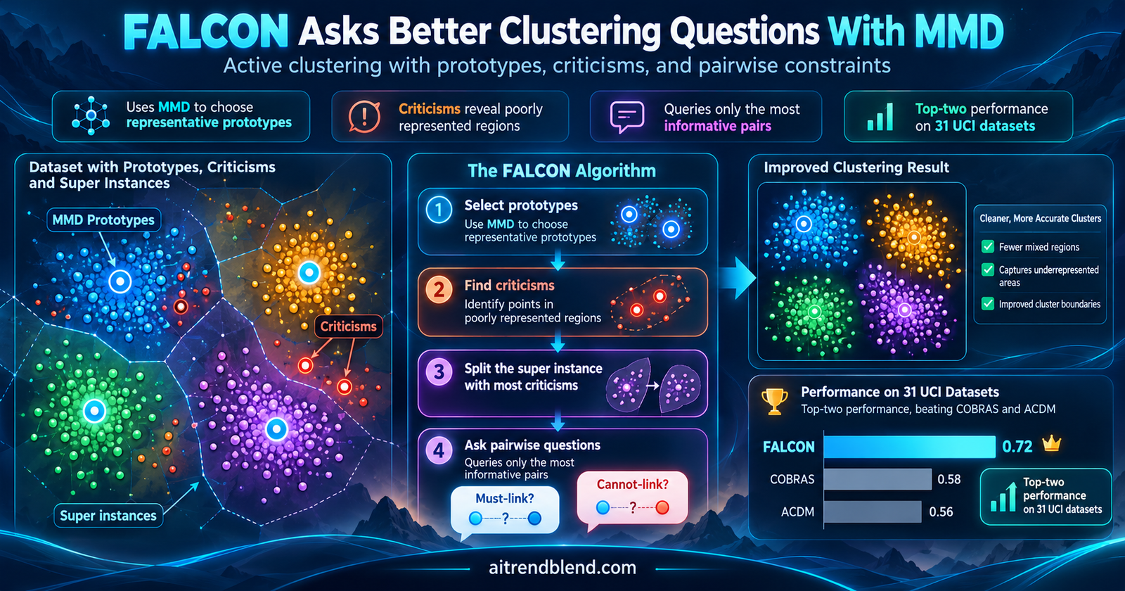
- FALCON picks a few prototypes that minimise the maximum mean discrepancy to the full dataset, then groups every point with its nearest prototype into super instances.
- Criticisms, points where the data has more mass than the prototypes account for, decide which super instance to split next. The user is only asked about the new pieces.
- On 31 UCI datasets with a simulated user, FALCON with a fixed kernel width had the best ARI at 30 percent of query budgets, against 19 percent for COBRAS and 27 percent for ACDM.
- Runtime is similar to COBRAS but far slower than ACDM on large data, at roughly 58 time units per query at 200 queries on the biggest sets, against under 1 for ACDM.
- Our checks suggest the formal submodularity guarantee rarely applies in practice, and a single kernel width of 0.25 may starve the method on high dimensional data. Both are fixable.
Why the choice of question is the whole problem
Unsupervised clustering has a well known weakness. Methods like k means and hierarchical clustering find the structure their assumptions allow, not necessarily the structure a domain expert means. Overlapping groups, noise and high dimensional features make the gap worse.
Semi supervised clustering closes that gap by injecting a little human knowledge. The lightest form of that knowledge is the pairwise constraint. A must link says two points belong in the same cluster. A cannot link says they do not. Nobody has to name the clusters or know how many there are. They only have to compare two items, which is something people do quickly and reliably.
The catch is arithmetic. A dataset with n points has about n squared over two possible pairs. At five thousand points that is roughly 12.5 million candidate questions, and the user will answer a few dozen. Random pairs are almost always uninformative, since most random pairs come from clusters that any algorithm would already separate. Active constraint based clustering is the study of picking the few pairs that actually change the answer.
Think about what this actually requires. A good question has to be about a part of the data that matters, which is a representativeness requirement. It also has to be about a part where the current clustering might be wrong, which is an uncertainty requirement. Most existing methods lean hard on one of the two. FALCON’s contribution is a single mathematical object that supplies both.
How earlier methods choose their questions
The most influential approach is COBRAS, from Van Craenendonck and colleagues. Its key move is the super instance, a small group of points believed to belong together, so a single question about two super instances constrains dozens of points at once. COBRAS starts with coarse super instances built by k means and keeps splitting them. When it needs to refine, it splits the largest super instance. Size is a sensible proxy for uncertainty, since big groups are more likely to hide two clusters. It is also a crude one, because a large, homogeneous cluster gets split repeatedly while a small, mixed region is ignored.
Uncertainty driven methods take the other path and query points near cluster boundaries, measured by entropy or similar scores. ACDM, from Fu and colleagues, runs diffusion over a sparse similarity graph and has a reputation for scaling well. SPACE from Zhou, Li, Wang and Zhang combines ensembles with self paced learning. These approaches are good at finding ambiguity but depend heavily on the initial partition and can neglect sparse regions entirely, which leads to redundant questions about the same contested border.
FALCON’s authors frame the gap in one sentence worth paraphrasing. Existing methods decide refinement from local uncertainty or cluster size, and almost none ask how well the current set of super instances covers the data distribution as a whole. If you have followed our earlier piece on what a cluster even is under Hartigan’s axioms, you will recognise the underlying tension. A clustering is a claim about where the probability mass lives, so judging it by distributional coverage is natural.
Measuring how well a few points stand in for the data
The maximum mean discrepancy, popularised for two sample testing by Gretton and colleagues, compares two distributions by mapping both into a reproducing kernel Hilbert space and measuring the distance between their mean embeddings. With a kernel \(k\), the squared MMD between distributions \(P\) and \(Q\) is
with \(X, X’\) drawn from \(P\) and \(Z, Z’\) from \(Q\). For a characteristic kernel, such as the Gaussian RBF, the MMD is zero only when the two distributions match. In empirical form, with \(n\) data points \(x_i\) and \(m\) candidate points \(z_j\), it becomes a sum of three kernel averages.
Here is the idea FALCON borrows from the MMD critic work of Kim and colleagues on interpretability. If you choose the \(z_j\) from the dataset itself, a small MMD means those few points form a faithful miniature of the whole. Those are prototypes. The points the miniature still misses are criticisms. Kim and colleagues used that pair to explain what a model had learned. FALCON uses it to decide where to ask questions.
Choosing prototypes
Dropping the first term of Equation 3, which does not depend on the prototypes, leaves a cost function to maximise over a prototype index set \(Pr\) of size \(m\).
The first term rewards prototypes that are close to many data points. The second penalises prototypes that are close to each other, so the set spreads out. The objective is linear in the kernel entries, and under conditions on the kernel matrix it is monotone submodular, which means a greedy forward algorithm that adds the best single point at a time reaches at least \(1 – 1/e\), about 63 percent, of the optimum. That is the classic Nemhauser, Wolsey and Fisher bound, and the paper notes, citing Feige, that no polynomial time method can do better in general unless P equals NP.
From prototypes to super instances
Each data point is then assigned to its nearest prototype in Euclidean distance, giving a partition into super instances.
Geometrically these are Voronoi cells around the prototypes. The difference from COBRAS is how the centres are chosen. K means centres minimise squared distance within groups. MMD prototypes minimise the mismatch between distributions, which tends to place representatives in proportion to where probability mass actually is.
Criticisms and the witness function
Here is where it gets interesting. The MMD has a natural pointwise companion, the witness function, which tells you at each location which distribution has more mass nearby.
With a Gaussian kernel, the first term is a smoothed density of the data around \(x\), and the second is a smoothed density of the prototypes. A large positive \(g(x)\) means the data are dense around \(x\) but the prototypes are not. A large negative value means a prototype sits somewhere the data are thin. Either way, \(x\) lives in a region the current summary describes badly.
FALCON picks \(m + 1\) criticisms, one more than the number of prototypes, by greedily maximising the summed absolute witness value plus a log determinant diversity term from the sensor placement work of Krause and colleagues.
Without the log determinant, the criticisms would pile up in the single most underserved spot. With it, the selection is pushed to spread across different problem areas. The extra criticism beyond \(m\) is there to break ties, so that if every super instance has one criticism, one of them still stands out.
Deciding what to split
The super instance that contains the most criticisms is split, with ties going to the larger super instance.
The number of criticisms inside it sets how many new local prototypes to add. Those prototypes are chosen with the same MMD objective, applied only to the points inside the chosen super instance, and then every point in the dataset is reassigned to its nearest prototype. Existing prototypes are never removed, so their count strictly grows each round and is bounded by n. The process has to terminate, and in the extreme every point becomes its own super instance.
Turning user answers into clusters
Clusters are built by merging super instances. For each new prototype, the existing clusters are sorted by distance from the prototype to the mean of the cluster’s prototypes.
The user is asked about the closest cluster first. A must link ends the search and the super instance joins that cluster. If every cluster gets a cannot link, a new cluster is created. Transitivity and entailment of constraints, as in the original COP k means work of Wagstaff and colleagues, avoid repeating questions whose answer is already implied.
FALCON does not ask where the clustering is uncertain. It asks where its own summary of the data is most wrong, and lets that answer double as uncertainty. aitrendblend analysis of FALCON, Information Fusion 2027
The paper’s worked example on a small two dimensional dataset shows the rhythm. FALCON starts with two prototypes and two super instances. One super instance holds two criticisms, so it is split into two new pieces, giving four. The user merges what belongs together. Next round, another super instance holds three criticisms, it is split into three, giving seven, and a final merge produces the three true clusters. The algorithm alternates between exploiting the current structure through merges and exploring underrepresented regions through splits.
What the experiments show
The evaluation is broad. FALCON was tested on 31 datasets from the UCI repository, ranging from 106 instances in Tae to 69,999 in MNIST, with between 2 and 26 classes. Duplicates and missing values were removed and every feature was scaled to the range zero to one. Constraints came from a simulated user who answered from the true class labels, which is standard in this literature.
Six baselines covered the main families. COBRAS and ACDM are the leading active methods. SPACE is an ensemble method. DBSSHC, from Jiang, Qin and Feng, is a density based semi supervised clustering method that uses randomly labelled data rather than queries. MPCKMeans-NPU is a constrained k means with neighbourhood based uncertainty and was given the true number of clusters, an advantage the other methods did not have. K means plus plus served as an unsupervised floor. Runs longer than 72 hours were stopped and excluded.
FALCON came in two configurations. The default uses a fixed RBF kernel width of 0.25 for both prototypes and criticisms. The best sigma version picks the width per dataset by exhaustive grid search, which the authors explicitly describe as an oracle style upper bound. The full results are in the FALCON paper in Information Fusion, which is open access.
Quality per question
The main metric is the adjusted rand index of Hubert and Arabie, which is 1 for a perfect match with the true labels and around 0 for random assignments. It was recorded after every query, so each method yields a learning curve rather than a single number. Averaged across all datasets, both FALCON curves sit above every baseline across the whole budget range, with the tuned version ending near 0.8 ARI at 500 queries and the default slightly below. A Wilcoxon signed rank test on paired ARI trajectories gives p values below 0.01, and the aligned rank comparison against COBRAS and ACDM returns p values in the region of 1e minus 34.
| Measure across all datasets and budgets | FALCON, sigma 0.25 | COBRAS | ACDM |
|---|---|---|---|
| Share of budgets with the best ARI | 30% | 19% | 27% |
| Share of budgets ranked first or second | 66% | 44% | 39% |
Table A. Win rates from the per dataset breakdown in the paper’s appendix. Datasets where FALCON did not rank first or second include Dermatology, Ionosphere and Pima.
The numbers tell a more measured story than the averaged curve. FALCON wins outright at less than a third of the evaluated budgets, and ACDM is close behind at 27 percent. What stands out is consistency. Two thirds of the time FALCON is in the top two, and the NDCG at rank 4 metric, which rewards staying near the top and punishes falling behind simple baselines, shows FALCON holding the highest score for most of the query range. The authors’ own conclusion is that FALCON is not the single best method everywhere but rarely falls out of the leading group, and that is a fair reading.
The shape of the curves matters too. COBRAS is strong in the very first queries, which makes sense because its coarse k means start is already a good partition. FALCON overtakes it quickly. ACDM starts weaker and improves late. FALCON also beats DBSSHC after only a handful of queries, which suggests that choosing what to ask beats labelling a random subset.
Runtime
| Dataset size | Method | 25 queries | 50 queries | 100 queries | 200 queries |
|---|---|---|---|---|---|
| Under 2,000 | FALCON | 0.42 | 1.07 | 2.69 | 9.86 |
| COBRAS | 2.70 | 3.62 | 5.23 | 7.1 | |
| ACDM | 0.33 | 0.31 | 0.42 | 0.63 | |
| 2,000 to 20,000 | FALCON | 36.7 | 77.4 | 145.49 | 318.15 |
| COBRAS | 50.06 | 96.33 | 171.18 | 305.92 | |
| ACDM | 4.5 | 4.05 | 4.07 | 4.66 | |
| Over 20,000 | FALCON | 2169.44 | 2835.91 | 5561.71 | 11674.49 |
| COBRAS | 1796.56 | 3587.08 | 7196.16 | 14078.95 | |
| ACDM | 164.71 | 161.12 | 163.46 | 160.18 |
Table B. Average runtime by dataset size and query budget, from Table 2 of Blase et al. The paper does not state the time unit, and seconds would be the natural reading.
FALCON and COBRAS are in the same league everywhere. ACDM is in a different one, nearly flat in the number of queries and one to two orders of magnitude faster on large data. Divide the totals by the query count and the interactive picture becomes clearer. On the largest datasets at 200 queries, FALCON averages roughly 58 units per question, COBRAS roughly 70 and ACDM under 1. If those units are seconds, a user of FALCON would wait about a minute between questions on a dataset the size of Skin or MNIST. On datasets under 2,000 points the wait is a fraction of a second, which is where the method is most comfortable today.
The authors are open about where the cost comes from. The full kernel matrix costs order n squared times d to build, once. Each round then selects criticisms in order r n m plus r cubed time and computes local prototypes inside the split super instance in order N cubed time, where N is that super instance’s size. They suggest kernel approximations, low rank embeddings and subsampling as remedies, and the earlier work we covered on fast kernel approximation by Dommel and Pichler is exactly the kind of tool that would help.
What drives the gains
Three analyses isolate the contribution of each idea. The first compares FALCON’s criticism driven choice of super instance with COBRAS’s rule of splitting the largest one, inside otherwise identical code. Criticism driven splitting gives higher average ARI across the whole range of 200 queries, ending around 0.68 against roughly 0.65 for the size rule. That supports the central claim directly. Where you refine matters, and distributional coverage is a better guide than size.
The second is an ablation. Replacing local MMD prototypes with randomly chosen local points, or removing refinement and criticisms altogether in favour of growing a global prototype set, both reduce ARI. Interestingly, dropping prototypes hurts more than dropping refinement. Refinement without good representatives is worse than good representatives without targeted refinement. The paper reads this as a sign that representativeness and uncertainty only work together, which fits the evidence.
The third swaps the kernel. A Laplacian kernel and a rational quadratic kernel, both characteristic, were tried in place of the Gaussian RBF. Neither matched it, and neither beat the ablated variants either.
The best supported result in the paper is not the headline win rate. It is the controlled comparison showing that splitting where criticisms concentrate beats splitting the biggest group, in the same framework. That idea is easy to transplant into other super instance based methods.
Sensitivity to the kernel width
The Gaussian kernel needs a width twice, \(\sigma_1\) for prototypes and \(\sigma_2\) for criticisms. An ANOVA across datasets found that only \(\sigma_1\) has a significant effect, and only in the early query stages, with p below 0.05. There was no interaction between the two. Among values from 0.025 to 10, a width of 0.25 for prototypes gave the best average curve, so the authors recommend using 0.25 for both.
What the paper does not settle
None of this comes for free, and three points deserve a closer look than the paper gives them.
The submodularity guarantee has demanding fine print. The approximation bound rests on the MMD objective being monotone submodular. The sufficient condition the paper quotes from the MMD critic work requires every off diagonal kernel value to be at most \(k_*/(n^3 + 2n^2 – 2n – 3)\), where \(k_*\) is the diagonal value. For a Gaussian kernel \(k_* = 1\). We worked out what that means.
| Dataset size n | Largest allowed off diagonal kernel value |
|---|---|
| 106, as in Tae | about 8.2e minus 7 |
| 1,000 | about 1.0e minus 9 |
| 69,999, as in MNIST | about 2.9e minus 15 |
Table C. The diagonal dominance condition from Corollary A.1.1, evaluated by the aitrendblend team. Every pair of distinct points would need near zero similarity.
A kernel that small between every pair of points carries almost no information about geometry, which is the opposite of what clustering needs. The authors say the condition is only sufficient and is relaxed because the number of prototypes is much smaller than n, and greedy selection often works well without a guarantee. Still, readers should treat the 63 percent bound as motivation rather than a property the experiments are known to enjoy.
One kernel width does not suit every dimension. After scaling features to the range zero to one, the typical squared distance between points still grows with the number of features. A width of 0.25 means the kernel divides squared distance by 0.125. We drew 300 random points uniformly in the unit cube and measured the median similarity between distinct points.
| Number of features | Example dataset size class | Median off diagonal RBF value at sigma 0.25 |
|---|---|---|
| 4 | Iris, Banknote | about 7e minus 3 |
| 34 | Ionosphere, Dermatology | about 4e minus 20 |
| 784 | MNIST | exactly 0 in floating point |
Table D. Kernel collapse with a fixed width, measured on uniform random data by the aitrendblend team. Real data are clumpier, so true values are larger, but the trend holds.
When the kernel is effectively zero between distinct points, every candidate prototype looks the same, the witness function is nearly flat, and the method’s distributional reasoning has little to work with. This is a hypothesis rather than a proven cause, but it lines up with the appendix plots, where higher dimensional sets such as MNIST show FALCON losing to COBRAS at many budgets. A width that scales with dimension, such as the median pairwise distance heuristic, would be a cheap thing to try and would not need labels. That matters, because the best sigma configuration chooses the width with exhaustive search that is only possible when you can score results against ground truth.
The simulated user never makes mistakes. Every constraint came from true labels. Real experts disagree, tire and misclick. Because FALCON merges greedily on the first must link and uses transitivity to skip questions, one wrong answer can propagate. The authors list noisy and conflicting constraints as future work, and until that test exists, the robustness claim refers to robustness across datasets, not robustness to the user.
If you try FALCON on your own data, set the kernel width from the data, for example with the median heuristic, rather than trusting 0.25 for every feature count. Expect interactive speeds below a few thousand points and plan for batch style sessions above that.
Where FALCON fits in a real workflow
The natural home for FALCON is a mid sized tabular dataset where labels are expensive but pairwise judgements are cheap. Think of a clinician grouping a few hundred patient profiles, a security analyst separating alert types, or a product team sorting support tickets into themes. In each case the expert can answer whether two items belong together far faster than they could write down a taxonomy.
The method has three practical advantages over its rivals. It does not need the number of clusters in advance, unlike constrained k means. It explains its choices, since prototypes and criticisms are actual data points a user can inspect. And it degrades gracefully, staying in the top two on most datasets even when it does not win.
It is less suitable when the data are very large or very high dimensional, for the runtime and kernel reasons above. It also assumes Euclidean geometry after scaling, so text or image data would first need a good embedding. That is the same caveat that applies to multi view spectral clustering methods like MST-WM, where the quality of the graph or kernel decides everything downstream.
There is a quieter lesson for anyone building interactive machine learning tools. FALCON shows that a well understood statistical object can do double duty. The MMD gives a summary and, through its witness function, a map of where that summary fails. Similar dual use shows up elsewhere, for example in prototype based graph classifiers such as HPGRL’s noise resistant prototypes. Choosing representatives and flagging what they miss are two sides of one calculation.
Limitations
Benchmark scope. All 31 datasets are tabular UCI sets with features scaled to the unit range. Many are small, with 20 of them under 1,000 instances. There are no text, image embedding or streaming scenarios, so performance on modern representation spaces is unknown.
Idealised supervision. The oracle is perfect and always available. Neither annotation noise nor a user who stops after a few questions mid session was studied.
Hyperparameter dependence. The default width was chosen by averaging across the same benchmark used for evaluation, and the best sigma results depend on label informed search. A truly label free width rule has not been tested.
Scalability. On datasets over 20,000 points, the runtime per query is high, and an ACDM style method is two orders of magnitude cheaper. The suggested speedups were not implemented or measured.
Reporting gaps. The runtime table has no units and is captioned as a dataset description. The appendix plots give per dataset comparisons only against COBRAS and ACDM. Variance across repeated runs is not shown for FALCON’s averaged curves. Our reconstruction below fills one gap by making each design choice explicit.
Reproducing FALCON in PyTorch
The code below is our independent reconstruction of Algorithm 1 from the paper’s equations. It is not the authors’ implementation, which is available on GitHub. It includes greedy MMD prototype selection, the witness function, greedy criticism selection with an incremental log determinant, criticism driven splitting with size as the tie break, nearest prototype super instances, a merge step that asks one question per candidate cluster, a simulated oracle and the adjusted rand index. Where the paper leaves a choice open we picked a default and commented it, such as asking each cluster about its prototype closest to the new one, and assigning a super instance to its nearest cluster without a question if the budget runs out mid merge.
On a synthetic set of 400 points in five unbalanced clusters, scaled to the unit square, our version reaches an ARI of 0.83 after 10 questions and about 0.95 after 25 and 50. The final lines of the smoke test reproduce the kernel collapse from Table D.
# FALCON reference implementation (aitrendblend reconstruction)
# Based on Blase, Aligon, Garouani, Ader and Teste, "FALCON, an effective and robust
# method for active clustering with pairwise constraints", Information Fusion 138 (2027) 104713.
# Independent reconstruction from the paper's equations and Algorithm 1, not the authors' code.
# Official code: https://github.com/VincentBlase/FALCON

import math
import torch


# ---------------------------------------------------------------------------
# 1. Kernel and MMD helpers (Eq. 1 to 3)
# ---------------------------------------------------------------------------
def rbf_kernel(A, B, sigma):
    """k(a, b) = exp(-||a - b||^2 / (2 sigma^2))"""
    d2 = torch.cdist(A, B).pow(2)
    return torch.exp(-d2 / (2.0 * sigma ** 2))


def mmd2(K_xx, K_xz, K_zz):
    """Biased empirical MMD^2 between X (n points) and Z (m points), Eq. 3."""
    n, m = K_xz.shape
    return K_xx.sum() / n ** 2 - 2.0 * K_xz.sum() / (n * m) + K_zz.sum() / m ** 2


# ---------------------------------------------------------------------------
# 2. Greedy prototype selection, maximise J_b(Pr) (Eq. 4 and 5)
# ---------------------------------------------------------------------------
def greedy_prototypes(K, m, candidates=None, existing=None):
    """
    K          : (n, n) kernel among the points of the region being summarised
    m          : number of prototypes to add
    candidates : boolean mask of points allowed as prototypes
    existing   : list of local indices already chosen (kept fixed)
    Returns the full list of chosen local indices.
    J(Pr) = 2/(n|Pr|) sum_i sum_{j in Pr} k(x_i, z_j) - 1/|Pr|^2 sum_{j,l in Pr} k(z_j, z_l)
    """
    n = K.shape[0]
    chosen = list(existing) if existing else []
    allowed = torch.ones(n, dtype=torch.bool) if candidates is None else candidates.clone()
    for c in chosen:
        allowed[c] = False
    col_sum = K.sum(dim=0)                                  # sum_i k(x_i, x_c)
    for _ in range(m):
        if not allowed.any():
            break
        p = len(chosen) + 1
        s1 = col_sum[chosen].sum() if chosen else torch.tensor(0.0)
        s2 = K[chosen][:, chosen].sum() if chosen else torch.tensor(0.0)
        cross = K[:, chosen].sum(dim=1) if chosen else torch.zeros(n)
        gain = 2.0 / (n * p) * (s1 + col_sum) - (s2 + 2.0 * cross + K.diagonal()) / p ** 2
        gain[~allowed] = -float("inf")
        best = int(torch.argmax(gain))
        chosen.append(best)
        allowed[best] = False
    return chosen


# ---------------------------------------------------------------------------
# 3. Witness function and criticism selection (Eq. 7 to 10)
# ---------------------------------------------------------------------------
def witness(K, protos):
    """g(x) = mean_i k(x, x_i) - mean_j k(x, z_j)   (Eq. 7)"""
    return K.mean(dim=1) - K[:, protos].mean(dim=1)


def greedy_criticisms(K, protos, n_crit, jitter=1e-6):
    """Maximise sum |g(w)| + log det K_{Cr,Cr} greedily over points that are not prototypes."""
    n = K.shape[0]
    g = witness(K, protos).abs()
    allowed = torch.ones(n, dtype=torch.bool)
    allowed[protos] = False
    chosen = []
    for _ in range(n_crit):
        if not allowed.any():
            break
        if chosen:
            K_cc = K[chosen][:, chosen] + jitter * torch.eye(len(chosen))
            K_xc = K[:, chosen]                              # (n, |Cr|)
            sol = torch.linalg.solve(K_cc, K_xc.T).T         # (n, |Cr|)
            resid = (K.diagonal() + jitter - (sol * K_xc).sum(dim=1)).clamp_min(1e-12)
        else:
            resid = K.diagonal() + jitter
        gain = g + torch.log(resid)                          # Schur complement update of log det
        gain[~allowed] = -float("inf")
        best = int(torch.argmax(gain))
        chosen.append(best)
        allowed[best] = False
    return chosen


# ---------------------------------------------------------------------------
# 4. Super-instances as nearest prototype cells (Eq. 6)
# ---------------------------------------------------------------------------
def assign_super_instances(X, protos):
    return torch.cdist(X, X[protos]).argmin(dim=1)           # index into protos


# ---------------------------------------------------------------------------
# 5. Pairwise oracle that simulates a user from ground truth labels
# ---------------------------------------------------------------------------
class Oracle:
    def __init__(self, labels):
        self.labels = labels
        self.queries = 0

    def must_link(self, i, j):
        self.queries += 1
        return bool(self.labels[i] == self.labels[j])


# ---------------------------------------------------------------------------
# 6. Merge a new prototype into existing clusters (Sec. 3.5, Eq. 13)
# ---------------------------------------------------------------------------
def merge_prototype(X, z, clusters, oracle, budget, cannot):
    """
    clusters : list of lists of prototype indices (global data indices)
    cannot   : dict proto -> set of cluster ids known to be cannot-link (entailment cache)
    Clusters are tried in order of distance to their mean prototype. Each cluster
    is asked once, using its prototype closest to z. A must link stops the search.
    """
    if not clusters:
        clusters.append([z]); return
    dists = [torch.norm(X[z] - X[c].mean(dim=0)).item() for c in clusters]
    for cid in sorted(range(len(clusters)), key=lambda c: dists[c]):
        if cid in cannot.setdefault(z, set()):
            continue                                         # already known, no query
        if oracle.queries >= budget:                         # out of queries, fall back
            nearest = min(range(len(clusters)), key=lambda c: dists[c])
            clusters[nearest].append(z); return              # to the closest cluster
        members = clusters[cid]
        rep = members[int(torch.cdist(X[z][None], X[members]).argmin())]
        if oracle.must_link(z, rep):
            members.append(z); return
        cannot[z].add(cid)
    clusters.append([z])                                     # no must link found


def labels_from_clusters(X, protos, clusters):
    owner = {p: cid for cid, c in enumerate(clusters) for p in c}
    si = assign_super_instances(X, protos)
    return torch.tensor([owner.get(protos[s], -1) for s in si.tolist()])


# ---------------------------------------------------------------------------
# 7. FALCON main loop (Algorithm 1)
# ---------------------------------------------------------------------------
def falcon(X, oracle, budget, sigma1=0.25, sigma2=0.25, n_init=2, log_every=10):
    n = X.shape[0]
    K1 = rbf_kernel(X, X, sigma1)                            # prototypes kernel, built once
    K2 = K1 if sigma2 == sigma1 else rbf_kernel(X, X, sigma2)  # criticisms kernel
    protos = greedy_prototypes(K1, n_init)                   # line 2
    clusters, cannot, history = [], {}, []
    for z in protos:                                         # line 4
        merge_prototype(X, z, clusters, oracle, budget, cannot)
    exhausted = set()

    while oracle.queries < budget and len(protos) < n:       # line 5
        si = assign_super_instances(X, protos)
        crits = greedy_criticisms(K2, protos, len(protos) + 1)          # line 6, m + 1
        counts = torch.bincount(si[crits], minlength=len(protos)).float()
        sizes = torch.bincount(si, minlength=len(protos)).float()
        for e in exhausted:
            counts[e] = -1.0
        # Eq. 12 with ties broken by super-instance size
        score = counts * (n + 1) + sizes
        split = int(torch.argmax(score))
        if counts[split] <= 0:
            break
        level = int(counts[split])                           # line 8
        local = torch.nonzero(si == split).squeeze(1)
        local_protos = [int((local == p).nonzero()) for p in protos if si[p] == split]
        cand = torch.ones(len(local), dtype=torch.bool)
        chosen = greedy_prototypes(K1[local][:, local], level, cand, local_protos)  # line 9
        new = [int(local[c]) for c in chosen[len(local_protos):]]
        if not new:
            exhausted.add(split); continue
        protos.extend(new)                                   # line 10, then line 11 next loop
        for z in new:                                        # line 12
            merge_prototype(X, z, clusters, oracle, budget, cannot)
        history.append((oracle.queries, labels_from_clusters(X, protos, clusters)))
    return labels_from_clusters(X, protos, clusters), protos, history


# ---------------------------------------------------------------------------
# 8. Adjusted Rand Index, the paper's main metric
# ---------------------------------------------------------------------------
def adjusted_rand_index(a, b):
    a = torch.unique(a, return_inverse=True)[1]
    b = torch.unique(b, return_inverse=True)[1]
    table = torch.zeros(int(a.max()) + 1, int(b.max()) + 1)
    table.index_put_((a, b), torch.ones(len(a)), accumulate=True)
    comb = lambda t: (t * (t - 1) / 2).sum()
    sum_ij = comb(table)
    sum_a, sum_b = comb(table.sum(1)), comb(table.sum(0))
    total = comb(torch.tensor(float(len(a))))
    expected = sum_a * sum_b / total
    max_idx = (sum_a + sum_b) / 2
    return float((sum_ij - expected) / (max_idx - expected + 1e-12))


# ---------------------------------------------------------------------------
# 9. Smoke test on synthetic clusters scaled to [0, 1], like the paper's preprocessing
# ---------------------------------------------------------------------------
if __name__ == "__main__":
    torch.manual_seed(0)
    centers = torch.tensor([[0.0, 0.0], [3.0, 0.5], [0.5, 3.0], [3.2, 3.0], [1.6, 1.6]])
    spreads = torch.tensor([0.35, 0.5, 0.3, 0.6, 0.25])
    sizes = [120, 80, 100, 60, 40]                           # unbalanced on purpose
    X = torch.cat([centers[i] + spreads[i] * torch.randn(s, 2) for i, s in enumerate(sizes)])
    y = torch.cat([torch.full((s,), i) for i, s in enumerate(sizes)])
    X = (X - X.min(0).values) / (X.max(0).values - X.min(0).values)   # min max scaling

    for budget in (10, 25, 50):
        oracle = Oracle(y)
        pred, protos, _ = falcon(X, oracle, budget=budget, sigma1=0.25, sigma2=0.25)
        print(f"budget {budget:3d}  queries used {oracle.queries:3d}  prototypes {len(protos):3d}"
              f"  clusters {int(pred.max()) + 1:2d}  ARI {adjusted_rand_index(pred, y):.3f}")

    # The kernel scale problem discussed in the article
    for d in (4, 34, 784):
        Z = torch.rand(300, d)
        K = rbf_kernel(Z, Z, 0.25)
        off = K[~torch.eye(300, dtype=torch.bool)]
        print(f"d = {d:3d}  median off diagonal kernel value {off.median():.2e}")
Two implementation notes. The full kernel matrix is built once, as in the paper, so memory grows with the square of the dataset size, which is fine for tens of thousands of points and not beyond. And because new prototypes never replace old ones, the prototype list doubles as an audit trail of every region the method chose to explore.
What FALCON adds to active clustering
FALCON’s core achievement is to give active clustering a principled way to decide where to look next. Instead of splitting the biggest group or querying the most ambiguous boundary, it summarises the data with MMD prototypes and refines wherever criticisms show that summary failing. On 31 UCI datasets, that strategy lands in the top two methods two thirds of the time and wins outright more often than COBRAS or ACDM.
The conceptual shift is in treating representativeness and uncertainty as one measurement rather than two competing heuristics. The witness function says, at every point, how much the current representatives underfit the data. Regions of high criticism density are where a single super instance is probably covering more than one cluster, and that is exactly where a question pays off.
The idea carries well beyond clustering. Any interactive system that keeps a compact summary of a dataset, whether for labelling, data cleaning, active learning for classification or dataset auditing, could use criticisms to decide what to show a human next. The same logic would help in summarising large document collections or picking which images a radiologist should review first, wherever a small set of examples has to stand in for a large one.
The limits are just as concrete. The formal approximation guarantee needs kernel conditions that are rarely met, a single fixed kernel width likely starves the method in high dimensions, runtime per question is too slow for interactive use on very large data, and the simulated user never errs. None of these undermine the experimental results. They mark where the method is ready and where it is not.
The next steps follow from that list. A label free kernel width rule, kernel approximations for large data, tests with noisy and inconsistent users and evaluation on learned embeddings for text and images. If those land, criticisms could become a standard ingredient in interactive clustering. For now, FALCON is a clear, well tested argument that the best question to ask is about the data your model understands least.
Frequently asked questions
What is FALCON in machine learning?
FALCON is an active constraint based clustering method. It asks a user whether pairs of items belong together and chooses those questions using prototypes and criticisms derived from the maximum mean discrepancy, so each answer improves the clustering as much as possible.
What are must link and cannot link constraints?
A must link constraint says two items belong in the same cluster, and a cannot link constraint says they belong in different clusters. They let a person guide clustering without naming the clusters or knowing how many there are.
How does FALCON differ from COBRAS?
Both group points into super instances and ask questions about them. COBRAS builds super instances with k means and splits the largest one. FALCON builds them around MMD prototypes and splits the one containing the most criticisms, the points its prototypes represent worst.
What are prototypes and criticisms?
Prototypes are a few real data points chosen so that their distribution matches the whole dataset as closely as possible under the MMD. Criticisms are points where the data have noticeably more or less mass than the prototypes suggest, marking regions the summary misses.
How well does FALCON perform?
Across 31 UCI datasets with a simulated user, FALCON with a fixed kernel width had the best ARI at 30 percent of query budgets and ranked first or second at 66 percent, compared with 19 and 44 percent for COBRAS and 27 and 39 percent for ACDM.
Is FALCON fast enough for large datasets?
On datasets under 2,000 points it is fast. On datasets above 20,000 points its runtime per query is similar to COBRAS but one to two orders of magnitude slower than ACDM, so very large data would need kernel approximation or subsampling.
Read the full FALCON paper
The open access article includes the full proofs, per dataset ARI tables for every budget and the sensitivity and ablation figures.
Blase, V., Aligon, J., Garouani, M., Ader, I., and Teste, O. (2027). FALCON, an effective and robust method for active clustering with pairwise constraints. Information Fusion, 138, 104713. doi.org/10.1016/j.inffus.2026.104713. Open access under CC BY NC 4.0.
This analysis is based on the published paper and an independent evaluation of its claims. Tables C and D, the per query runtime figures and the PyTorch code are the aitrendblend team’s own work. All other figures are taken from the paper, with curve values read approximately from its plots.